Action-Amplitude Approach to Controlled Entropic Self-Organization

Abstract

Motivated by the notion of perceptual error, as a core concept of the perceptual control theory, we propose an action-amplitude model for controlled entropic self-organization (CESO). We present several aspects of this development that illustrate its explanatory power: (i) a physical view of partition functions and path integrals, as well as entropy and phase transitions; (ii) a global view of functional compositions and commutative diagrams; (iii) a local geometric view of the Kähler–Ricci flow and time-evolution of entropic action; and (iv) a computational view using various path-integral approximations.

1. Introduction

We are primarily interested in developing advanced models of military command and control (C2), which we formulate (in its simplest form) as follows. Our approach should also be applicable across a wide range of non-military organizational decision-making settings. Consider a group Γ := {Γ_i: i = 1, 2, …, n} of n agents, each characterized by its own intent, I_i, and the set of m capabilities {C_j: j = 1, 2, …, J}. The basic modelling construction of the problem is that, according to perceptual control theory (see [1,2]), the perceptual error of an agent, Γ_i, is the difference between its intent and the consequences of its choice of a capability, C_j:

$$E_i=|I_i-A_i(C_j)|.$$

(1)

Thus, under this construction, the optimal behavior, ${\Gamma }_i^{{}^{opt}}$, of each agent, Γ_i, is given by minimizing the perceptual error, E_i:

$${\Gamma }_i^{{}^{opt}}=\underset{C_j}{min}(E_i),$$

(2)

so that the probability Pr_i = Pr_i(X_i = C_j) of a specific choice, C_j, is expected to be maximal when the perceptual error (2) is minimal.

(1)

The following geometrical interpretations can be given to the optimization Problem (1) and (2): (1) The perceptual error, E_i, given by the simple absolute value (1) can be “promoted” to the Euclidean L²-norm:

$$E_i^{\text{nrm}}=\parallel I,A\parallel =\sqrt{{\displaystyle \sum _{i=1}^n|}{I}_i-A_i(C_j){|}^2},$$

(3)

or to the Euclidean metric:

$$E_i^{\text{mtr}}=\mathrm{d}(I,A)=\sqrt{{\displaystyle \sum _{i=1}^n[I_i^2-A_i^2(C_j)]}}.$$

(4)

(2)

Its continuous generalization, allowing for a continuum of capability choices, is given by the Banach L²-norm:

$$B_i^{\text{nrm}}=\parallel [I,A]\parallel =\sqrt{{\displaystyle {\int }_a^b|I(x)-A[C(x)]{|}^{2}dx}},$$

(5)

and the associated Banach metric between any two real-valued square-integrable functions, I, A, defined on a real interval, [a, b] ⊂ ℝ:

$$B_i^{\text{mtr}}=\mathrm{d}(I,A)=\sqrt{{\displaystyle {\int }_a^b|I{(x)}^2-g{(x)}^2|dx}.}$$

(6)

For example, the finite control problem is actually a minimization of the square of the Banach metric (6). (We remark that in finite control (i.e., output tracking and navigation), we want the scalar system output, y(x, t), to follow a continuous nominal objective trajectory, say χ(t), for a given MD system vector, x, and where t is time. This problem can be expressed as:

$$\underset{\mathrm{x}\in {ℝ}^M}{min}{\displaystyle {\int }_{t_0}^{t_1}{[y(\mathrm{x},t)-\mathrm{\chi }(t)]}^{2}dt.}$$

Upon time discretization using a suitable quadrature scheme, this becomes the following least-squares problem:

$$\underset{\mathrm{x}\in {ℝ}^M}{min}f(\mathrm{x})={\displaystyle \sum _{i=1}^N{[\tilde{y}(\mathrm{x},t_i)-\tilde{\chi }(t_i)]}^{2}dt}.$$

Both discretized functions, $\tilde{y}(\mathrm{x},t_i)$ and $\tilde{\chi }(t_i)$, include the weights of the chosen quadrature scheme.)

(3)

The optimization Problem (2) can be rewritten in variational formulation as the stationary Hamilton action problem:

$$\delta E_i=0,$$

with the following particular cases:

$$\begin{array}{rrr}\hfill \delta \left|I_i-A_i(C_j)\right|=0& \hfill \text{or}& \hfill \delta |I(x)-A[C(x)]|=0,\\ \hfill \delta \sqrt{{\displaystyle \sum _{i=1}^n|I_i-A_i(C_j){|}^2}}=0& \hfill \text{or}& \hfill \delta \sqrt{{\displaystyle {\int }_a^b|}I(x)-A[C(x)]{|}^{2}dx=0,}\\ \hfill \delta \sqrt{{\displaystyle \sum _{i=1}^n[I_i^2-A_i^2(C_j)]}}=0& \hfill \text{or}& \hfill \delta \sqrt{{\displaystyle {\int }_a^b|}I{(x)}^2-g{(x)}^2|dx=0.}\end{array}$$

From these cases, the set of discrete Euler–Lagrangian equations of motion on the group/graph, Γ, can be derived (see [3], as well as Section 3 below). Geometrically, this means that the perceptual error, in all three forms—the absolute value (1), the L²-norm (3)–(5), or the metric (4)–(6)—represents an energy landscape. The optimization problem is some kind of a gradient or Levenberg-Marquardt (LM) descent along the Lagrangian geodesics of this energy landscape. (Note that the LM-algorithm, sometimes also known as “damped least squares” (DLS), interpolates between the gradient descent and the Gauss-Newton algorithm for quick and efficient convergence, by properly adjusting the damping parameter. It is more robust than Gauss-Newton, meaning that it can often find an optimum even when initialized far from it.)

Next, we assume the probability Pr_i = Pr_i(X_i = C_j) of a specific choice, C_j, in the optimization Problem (1) and (2) to be a monotonically-decreasing function of the perceptual error, E_i$\text{(or}{E}_i^{\text{nrm}}-B_i^{\text{nrm}}\text{or}{E}_i^{\text{mtr}}-B_i^{\text{mtr}})$. if we consider only a finite set of capabilities, a useful example of the probability distribution function (PDF) can be formulated as an exponentially-weighted collection of discrete Dirac-delta functions:

$$\underset{i}{\mathrm{Pr}}(X_i=C_j=\delta |I_i-A_i(C_j)|e^{-\beta E_i}.$$

(7)

The PDF (7) can be easily generalized to the Gibbs measure of a random variable, X_i, having the set of corresponding coordinates, {xⁱ}, defined by the PDF [4]:

$$\mathrm{Pr}(X_i=x^i)=\frac{1}{Z(\beta )}{\mathrm{e}}^{-\beta H(x^i)}\equiv \frac{\exp [-\beta H(x^i)]}{{\sum }_{x^i}\exp [-\beta H(x^i)]},$$

where $H=H(x^i)\equiv E_i(\text{or}H\equiv E_i^{\text{mtr}},\text{or}H\equiv E_i^{\text{nrm}})$ is the Hamiltonian energy function of the above energy landscape with local coordinates, {xⁱ}, and β is a free parameter (in thermodynamics, β would be inverse temperature). The corresponding partition function (see, e.g., [5]):

$$Z(\beta )={\displaystyle \sum _{x^i}{e}^{-\beta H(x^i)}}$$

(8)

provides the Gibbs measure on the system’s state-space, which is a unique statistical distribution that maximizes the entropy for a fixed expectation value of the energy:

$$\langle H(x^i)\rangle =-\frac{\partial \log (Z(\beta ))}{\partial \beta }.$$

The associated system’s order parameter, entropy, is given by:

$$S=-{\displaystyle \sum _{x^i}P(x^i)\ln P(x^i)=\beta \langle H(x^i)\rangle }+\log Z(\beta ).$$

Entropy describes both “ignorance”, or Heisenberg’s uncertainty, and “randomness”.

A useful particular example of Equation (8) is the partition function of a three-dimensional ensemble of n “molecules”, given by the 6n-dimensional phase-space integral:

$$Z(\beta )={\int }_{{ℝ}^{6n}}\exp [-\beta H(x^i)]d^3{p}_i{d}^3{x}^i,$$

(9)

where p_i = p_i(xⁱ) are generalized momenta.

More generally, we consider Markov random fields/Markov networks, which have a Markov property described by an undirected graph (see [4]). In Markov networks with local vertex coordinates, {xⁱ}, the PDF is usually given by the log-linear inner product model:

$$\underset{i}{\mathrm{Pr}}(X_i=x^i)=\frac{1}{Z}\exp \left({\displaystyle \sum _{i=1}^n{w}_i{f}_i}\right),$$

(10)

where f_i = f_i(xⁱ) are the feature functions and w_i are their corresponding weights (so that ∑ w_if_i is their dot-product), while Z is the partition function. When the PDF (10) is strictly positive, the Markov network is often called the Gibbs random field.

We remark here that Markov random fields have been introduced as a Markovian framework for the Ising spin-lattice model, defined by the Hamiltonian energy function (given here in its simplest dot-product form):

$$H(\sigma )=-{\displaystyle \sum _{i=1}^n{\displaystyle \sum _{i=1}^n{J}_{ij}{\sigma }_i{\sigma }_j,}}$$

where σ_i ∈ {+1, −1} are discrete spin-up and spin-down states (or, more generally, Pauli spin matrices), while J_ij is the interaction matrix with synaptic weights. The same Hamiltonian has also been used in Hopfield neural networks [6], in which case, σ_i represents the state of the McCulloch–Pitts neuron [7].

In this paper, we present several different views of an action-amplitude model for controlled entropic self-organization (CESO).

2. Physical View on CESO

2.1. From Partition Function to Feynman’s Path Integral

We have already seen from example Equation (9) that the number of random variables, X_i, need not be countable; if we continue in this direction, the set of corresponding coordinates, {xⁱ}, becomes a field ϕ = ϕ (x) ∈ ℝⁿ. Consequently, the sum in Equation (8) is replaced by the path integral (see, e.g., [8]):

$$Z(\varphi )={\displaystyle \int D[\varphi ]{\mathrm{e}}^{-\beta H(\varphi )}},$$

(11)

where D[ϕ] represents the appropriate Lebesgue measure. (We remark that as any quantum system has both a continuous spectrum (consisting of eigenfunctions) and a discrete spectrum (consisting of eigenvectors), the path-integral symbol, ∫ D[ϕ], represents both the integration over the continuous spectrum and the summation over the discrete spectrum of the field system ϕ = ϕ (x) [8].)

More generally, in quantum field theory, instead of the field Hamiltonian, H(ϕ), we have the classical (Lagrangian or Hamiltonian) action, A(ϕ), of the theory. Both the real path integral in imaginary time (the so-called Euclidean path integral):

$$Z_{\mathrm{Euc}}(\varphi )={\langle \text{out}|\text{in}\rangle }_{\mathrm{Euc}}={\displaystyle {\int }_{{ℝ}^n}D[\varphi ]{\text{e}}^{-A[\varphi ]},}$$

(12)

and the complex path integral in real time (the so-called Lorentzian path integral):

$$Z_{\mathrm{Lor}}(\varphi )={\langle \text{out}|\text{in}\rangle }_{\mathrm{Lor}}={\displaystyle {\int }_{{ℝ}^n}D[\varphi ]{\text{e}}^{iA[\varphi ]},}$$

(13)

represent partition functions of the quantum field theory in ℝⁿ. In both cases, quantum probability Pr(ϕ) is defined as the absolute square of the transition amplitude:

$$\mathrm{Pr}(\varphi )=|\langle \text{out}|\text{in}\rangle {|}^2.$$

Finally, we generalize our quantum theory of fields, from ϕ ≡ ϕ (x) ∈ ℝⁿ to Φ ≡ Φ(x) ∈ M, defined on an arbitrary nonlinear configuration, n-manifold M, with its curved geometry and topology with a certain number of holes. In this way, we arrive at our main conceptual tool, the geometrical/topological path integral, in its Euclidean and Lorentzian versions, respectively given by (see [3]):

$$\begin{array}{l}{Z}_{\mathrm{Euc}}(\Phi )={\langle out|in\rangle }_{\mathrm{Euc}}{}_{(M)}={\displaystyle {\int }_{M}D[\Phi ]{\text{e}}^{-A[\Phi }{}^{]},}\hfill \\ Z_{\mathrm{Lor}}(\Phi )={\langle out|in\rangle }_{\mathrm{Lor}}{}_{(M)}={\displaystyle {\int }_{M}D[\Phi ]{\text{e}}^{\text{i}A[\Phi ]}.}\hfill \end{array}$$

(14)

Here, A[Φ] represents classical Lagrangian action, the integration is performed over all continuous paths + fields + geometries defined on the configuration manifold, M, while summation is performed along the edges of the corresponding discrete graph structure, obtained either by putting the tram-tracks-like constraints along the manifold, M, or by performing some form of triangulation discretization. (Note that, given any topological/smooth manifold, M, one can always obtain not one, but rather a family (or a set) of discrete network/graph structures on it, defined either by fixing some tram-like constraints of motion or by simplicial (or Regge-type) triangulation. In terms of dynamics, this means spatio-temporal discretization (e.g., from the standard continuous Laplacian (or Laplace–Beltrami) operator, △, defined on a manifold, M, one can obtain the discrete Laplacian, △_d.))

2.2. Three-Phase Entropic Framework with Transition Amplitudes

Recall that Prigogine’s Extended Second Law of Thermodynamics [9]:

$${\partial }_{t}S\ge 0,(\text{where}{\partial }_{t}S\equiv \partial S/\partial t),$$

(15)

considers open (i.e., non-isolated) irreversible systems or processes that exchange energy and matter with their environment in such a way that the entropy change (or entropy variation) is given by the sum of the internal and external entropy changes:

$${\partial }_{t}S=\frac{d_{i}S}{dt}+\frac{d_{e}S}{dt},$$

(16)

where d_iS denotes the internal entropy production within the system, while the d_eS is the external entropy flux, due to the exchanges with the environment. For an isolated system, d_eS = 0.

By further extending Prigogine’s open Second Law (15) into the strict-control regime, we formulate a generic three-phase entropic framework for entropy, S, in any complex system described by one of the partition functions (11)–(14). The framework consists of the following components:

(1)

The phase of Intent, given by the monotonically increasing entropy: ∂_tS > 0;

(2)

The phase of Action, corresponding to the conservation of information, described by the conserved entropy: ∂_tS = 0;

(3)

The phase of Control, described by the monotonically decreasing entropy: ∂_tS < 0.

The phase transition from one phase to another, caused by the system’s topology change (see [8]), is described by the transition amplitude:

$$\langle {\text{out phase}}_{t_1}|{\text{in phase}}_{t_0}\rangle :={\displaystyle {\int }_{{\text{tch}}_d^c(M)}D[\Phi ]{\text{e}}^{\text{i}A[\Phi ]},}$$

where “ ${\text{tch}}_d^c(M)$” denotes both continuous topology change “ ${\text{tch}}^c(M)$” of the system’s configuration manifold, M, and discrete topology-change “ ${\text{tch}}_d(M)$” of the system’s configuration graph/network structure (e.g., removing or adding vertices of the graph).

3. Global Functional View on CESO

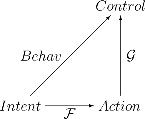
The set—or, more appropriately, the category—of generic agents’ behaviors, Behav, is defined by the functional composition of the following two successive multidimensional maps:

such that the following diagram commutes:

The maps, F and G, are given by their respective adaptive path integrals, meaning partition functions defined by the respective multi-phase and multi-path (multi-field and multi-geometry) transition amplitudes:

$$F:Inten{t}_{t_0}\to Actio{n}_{t_1}:=\stackrel{{\partial }_{t}S=0}{\langle Actio{n}_{t_1}}|\stackrel{{\partial }_{t}S>0}{Inten{t}_{t_0}\rangle }={\displaystyle {\int }_{\text{tch}(M)}D[w\Phi ]{\text{e}}^{\text{i}{A}_1[\Phi ]},}$$

(17)

$$G:Actio{n}_{t_1}\to Contro{l}_{t_2}:=\stackrel{{\partial }_{t}S<0}{\langle Contro{l}_{t_2}}|\stackrel{{\partial }_{t}S=0}{Actio{n}_{t_1}\rangle }={\displaystyle {\int }_{\text{tch}(M)}D[\omega \Psi ]{\text{e}}^{\text{i}{A}_2[\Psi ]}.}$$

(18)

Here, the Lebesgue integration, in both integrals, is performed over all continuous $({\Phi }_c^i,{\Psi }_c^i)$ = paths + fields + geom/topologies, while summation is performed over all discrete random processes (i.e., Markov chains) and regional network-topologies, $({\Phi }_d^j,{\Psi }_d^j)$.

The path integral Equations (17) and (18) are constructed, respectively, from the classical behavioral actions (see [3]):

(19)

(where the overdot denotes the time derivative) and their corresponding action principles:

$$\begin{array}{ccc}\delta A_{\text{1}}\left[\Phi \right]=0& \text{and}& \delta A_{\text{2}}\left[\Phi \right]=0.\end{array}$$

These correspond to classical Euler–Lagrangian equations of motion on the configuration manifold, M, with the Riemannian metric tensor, g_ij:

$$\begin{array}{ccc}\frac{d}{dt}{L}_{{\dot{x}}^i}=L_{{\dot{x}}^i}& \text{and}& \frac{d}{dt}{\mathfrak{L}}_{{\dot{x}}^i}={\mathfrak{L}}_{{\dot{x}}^i}\end{array}$$

with Lagrangians:

$$\begin{array}{ccc}L=\frac{1}{2}{g}_{ij}{\dot{x}}^i{\dot{x}}^j-\Phi (x^i)& \text{and}& \mathfrak{L}=\frac{1}{2}{g}_{ij}{\dot{x}}^i{\dot{x}}^j-\Psi (x^i)\end{array}.$$

The symbolic differentials, D[wΦ] and D[ωΨ], in the path integral Equation (17) represent adaptive path measures, defined as the weighted products:

$$\begin{array}{cc}D[w\Phi ]=\underset{N\to \infty }{\lim }{\displaystyle \prod _{s=1}^N{w}_{s}d{\Phi }_s^i,}& (i=1,\dots ,N=co{n}_i+di{s}_i),\\ D[\omega \Psi ]=\underset{M\to \infty }{\lim }{\displaystyle \prod _{p=1}^M{\omega }_{p}d{\Psi }_s^k,}& (k=1,\dots ,M=co{n}_k+di{s}_k).\end{array}$$

Both adaptive path integral Equations (17) and (18) represent arbitrary topology ∞-dimensional neural networks (see [10]), with weights (w, ω) updated according to:

$$\begin{array}{cc}w(t+\text{1})=w(t)+Inno{v}^w(t),& \omega (t+\text{1})=\omega (t)+Inno{v}^{\omega }(t),\end{array}$$

where Innov^w(t) and Innov^ω(t) are their respective innovations.

4. Local Geometric View on CESO

A complexified extension of the behavioral action Equation (19), which is more appropriate for general Lorentzian path integrals, is called the Kähler-Perelman entropic action, W(g), that is, roughly speaking, a complexified Einstein–Hilbert action from general relativity. In this section, we present its time-evolution along the complex geometric dynamics, called the Kähler-Ricci flow. For this objective, we utilize the richest and most useful structure in the Kähler geometry, the so-called Fano manifold, which is a compact (i.e., closed and bounded) Kähler n-manifold (M, g) with positive first Chern class c₁(M).

Recall that a Kähler manifold (M, g) is a complex n-manifold that has the following basic characteristics (for a recent review, see [11] and the references therein):

(1)

A set of n local holomorphic coordinates: {z₁, · · ·, z_n} ∈ U ⊂ M, with the corresponding complex-valued differentials:

$$\begin{array}{cc}d{z}_k=d{x}_k+\mathrm{i}d{y}_k,& d{\overline{z}}_k=d{x}_k-\mathrm{i}d{y}_k;\end{array}$$

(2)

Hermitian metric tensor: $g_{i\overline{j}}=g_{i\overline{j}}(z^i,z^{\overline{j}})$, with the corresponding Kähler metric, g, as a positive and symmetric (1,1)-form:

$$g=\mathrm{i}{g}_{i\overline{j}}d{z}^i\otimes d{z}^{\overline{j}},$$

and the associated Kähler form, ω, as a closed (dω = 0) and positive (1,1)-form:

$$\omega =\mathrm{i}{g}_{i\overline{j}}d{z}^i\wedge d{z}^{\overline{j}};\text{ and}$$

(3)

Functional space of Kähler potentials:

$$P=\left\{\phi \right|{\omega }_{\phi }=\omega +\text{i}\partial \overline{\partial }\phi >0\}.$$

Now, consider the normalized Kähler–Ricci flow on a Fano n-manifold (M, g):

$$\begin{array}{cc}{\partial }_{t}g(t)=g(t)-\text{Ric}[g(t)])& ({\partial }_t\equiv \partial /\partial t).\end{array}$$

(20)

In a local open chart U ⊂ (M, g), starting from some smooth initial Kähler metric $g_0=g_{i\overline{j}}(0)$ flow Equation (20) is given by:

$$\begin{array}{cc}{\partial }_t{g}_{i\overline{j}}(t)=g_{i\overline{j}}(t)-R_{i\overline{j}}(t),& (\text{for}i,j=1,\dots ,n)\end{array}.$$

We remark here that of central importance in Kähler geometry are the so-called Dolbeault differential operators: ∂ ≡ ∂_j and $\overline{\partial }\equiv {\partial }_{\overline{j}}.$ Any p-form α defined on the Kähler manifold (M, g) is called $\overline{\partial }$-closed iff $\overline{\partial }\alpha =0$ and $\overline{\partial }$-exact iff $\alpha =\overline{\partial }\eta$ for some (p − 1)-form η on (M, g). The Dolbeault cohomology group $H_{\overline{\partial }}^{1,1}$ (M, ℝ) is a complexification of the standard de Rham cohomology group $H_d^2$(M,ℝ), defined on (M, g) as a quotient:

$$H_{\overline{\partial }}^{1,1}(M,ℝ)=\frac{\{\overline{\partial }\text{-closed real}(1,1)\text{-forms}\}}{\{\overline{\partial }\text{-exact real}(1,1)\text{-forms}\}}.$$

It was proven in [12] that Equation (20) has a global solution, g(t), in the case that g₀ has canonical Kähler class, i.e., 2πc₁(M) as its Kähler class. In particular, by the $\partial \overline{\partial }$-lemma, there exists a family of real-valued functions, u(t), called Ricci potentials (see, e.g., [13]) of the metric, g(t), which are special Kähler potentials. They are determined by:

$$\begin{array}{cc}{g}_{i\overline{j}}-R_{i\overline{j}}={\partial }_i{\partial }_{\overline{j}}u,& \frac{1}{V}{\displaystyle {\int }_M{e}^{-u(t)}d{v}_{g(t)}=1,}\end{array}$$

Where $V={\displaystyle \int d{v}_g}$ denotes the volume of the Kähler–Ricci flow. (The corresponding evolutions of the Ricci curvature $R_{i\overline{j}}=R_{i\overline{j}}(t)$ and the scalar curvature R = R(t) on the Kähler manifold (M, g) are governed, respectively, by:

$$\begin{array}{l}{\partial }_t{R}_{i\overline{j}}+{\Delta }_M{R}_{i\overline{j}}+R_{i\overline{j}p\overline{q}}{R}_{p\overline{q}}-R_{i\overline{p}}{R}_{p\overline{j}},\\ {\partial }_{t}R={\Delta }_{M}R+R_{i\overline{j}}{R}_{j\overline{i}}-R,\end{array}$$

(21)

starting from some smooth initial Ricci and scalar curvatures, $R_{i\overline{j}}$(0) and R(0), respectively.)

From the control-theory perspective, the most important characteristic of the Kähler-Ricci flow is the existence of its solitary solutions (solitons), which are shrinking or decaying in time. This characteristic is associated with the geometrical entropy decrease and gives the global Lyapunov stability to the flow.

Formally, a Riemannian manifold (M, g) represents a shrinking Ricci soliton iff (see, e.g., [13]):

$$\begin{array}{cc}\text{Ric}(g)+\text{Hess}(u)=\mathrm{\lambda }g,& (\mathrm{\lambda }>0)\end{array}.$$

In particular, if (M, g) is a Fano manifold with g ∈ 2πc₁(M), it is a shrinking Kähler-Ricci soliton iff λ = 1 and u ≡ u(t) is the Ricci potential; that is, iff (see [11] and references therein):

$$\nabla \nabla u=0,$$

or, applying the Bianchi identity, iff the following Schur-identity holds:

$$\nabla u-|\nabla u{|}^2+u=a.$$

For any Kähler metric, g ∈ 2πc₁(M), with scalar curvature s and any smooth real time-function u ≡ u(t), define the Kähler–Perelman entropy E ≡ E(g) defined by the following infimum of sets of entropy functionals (compare with Perelman’s original definition [14]):

$$\begin{array}{l}\begin{array}{cc}\epsilon (g)=\inf \left\{W(g,u):{\displaystyle {\int }_M{\mathrm{e}}^{-u}dv=V}\right\},& where\end{array}\\ W(g,u)=\frac{1}{V}{\displaystyle {\int }_M(s+|\Delta u{|}^2+u-n){\mathrm{e}}^{-u}dv.}\end{array}$$

A smooth minimizer of the entropy, ε, always exists, though it need not necessarily be unique (see [15]). Entropy ε admits a natural upper bound:

$$\epsilon (g)\le \frac{1}{V}{\displaystyle {\int }_{M}u{\mathrm{e}}^{-u}dv=a\le 0.}$$

To see how the Kähler–Perelman entropic action, W(g, u), evolves under the Kähler-Ricci flow (20), recall that for any solution, u(t), of the backward heat equation (compare with [14]):

$${\partial }_{t}u=-\Delta u+|\nabla u{|}^2+\Delta u,$$

(22)

we have:

$${\partial }_{t}W(g,u)=\frac{1}{V}{\displaystyle {\int }_M[|\nabla \overline{\nabla }(u-u){|}^2+|\nabla \nabla u{|}^2]}{\mathrm{e}}^{-u}dv,$$

which implies the Kähler-Perelman monotonicity condition on the geometric entropy [11]:

$$\begin{array}{cc}(\forall t\ge 0),& \epsilon (g_0)\le \epsilon [g(t)]\le 0.\end{array}$$

Roughly speaking, the application of control is trying to reduce the system’s entropy. This is achieved through shrinking Kähler-Ricci solitons.

5. Computational View on CESO

In this section, we will outline a fast desktop simulation framework for controlled entropic self-organization, based on the preceding idea of the functional composition of path-integrals Equations (17) and (18).

In quantum field theory, there is both a theoretical and a numerical approach to solve a similar path integral as a sum-over-fields. A theoretical way consists of its perturbative expansion into a series of Feynman diagrams; although there is a Mathematica^® package, FeynArts–FeynCalc, devoted to this, this approach does not scale well with respect to increasing numbers of agents and, therefore, is not well suited to our task. A numerical way of handling the problem might be to discretize a path integral on a lattice (of dimension two, three or four) and use the techniques of lattice gauge theory; again, although possible, this approach is not really feasible for the numbers of agents in which we are typically interested. (We remark that military command and control (C2) can involve hundreds of actors, and it is not unreasonable to expect that other non-military decision-making processes could involve similarly large numbers.)

In non-relativistic quantum mechanics, the path integral can be numerically solved, either by a direct implementation of the Feynman formula (see, e.g., [16]) or by Monte Carlo methods. Both these kinds of solvers are fairly slow, except for the Metropolis algorithm [17]. As shown in Feynman’s first paper [18], this path integral is equivalent to the linear Schrödinger equation. Its adaptive version is equivalent to the cubic nonlinear Schrödinger equation (NLS; see [19] and the references therein).

By analogy, in statistical mechanics, the real path integral in real time is equivalent to the linear Fokker-Planck equation, while its adaptive version is equivalent to the nonlinear Fokker-Planck equation. This approach is developed in the next subsection.

5.1. Fokker–Planck–Ito Approach

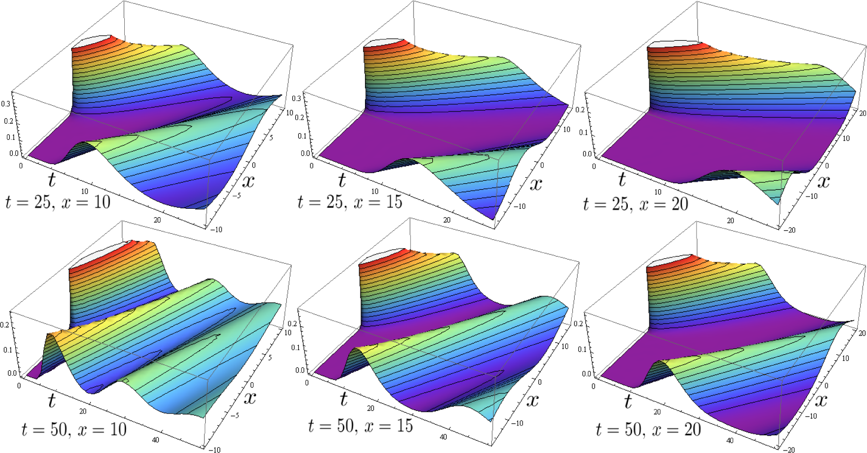
The Fokker–Planck equation, also known as the Kolmogorov forward equation:

$$\begin{array}{c}{\partial }_{t}P(x,t)=-{\partial }_x[f(x,t)P(x,t)]+\frac{1}{2}{\partial }_{xx}[g^2(x,t)P(x,t)]\\ =[-{\partial }_{x}f(x,t)+\frac{1}{2}{\partial }_{xx}{g}^2(x,t)P(x,t)]\end{array}$$

(23)

is a parabolic partial differential equation (PDE) that describes the time-forward evolution of the probability distribution, P (x, t), also called the probability density function (PDF; see Figure 1). The expression on the right-hand side of Equation (23), including:

$$\begin{array}{c}\begin{array}{cc}\text{linear advective term}:-{\partial }_{x}P\left(x,t\right)f\left(x,t\right),& \text{and}\end{array}\\ \text{quadratic diffusive term }:\frac{1}{2}{g}^{\text{2}}\left(x,t\right){\partial }_{xx}P\left(x,t\right),\end{array}$$

defines the Fokker-Planck differential operator:

$$D_{FP}:=-{\partial }_{x}f(x,t)+\frac{1}{2}{\partial }_{xx}{g}^2(x,t).$$

Note that the quadratic diffusive term vanishes in the case of zero noise g(x, t) = 0.

The PDE (23) satisfies the probability conservation law:

$${\partial }_{t}P(x,t)+{\partial }_{x}J(x,t)=0$$

where J(x; t) represents the probability current, defined as:

$$J(x,t):=f(x,t)P(x,t)-\frac{1}{2}{\partial }_{x}g(x,t)P(x,t).$$

(Note that the backward Fokker–Planck equation or the Kolmogorov backward equation:

$$\begin{array}{l}{\partial }_{t}P(x,t)=-f(x,t){\partial }_{x}P(x,t)-\frac{1}{2}{g}^{\text{2}}(x,t){\partial }_{xx}P(x,t)\\ =-[f(x,t){\partial }_x+\frac{1}{2}{g}^{\text{2}}(x,t){\partial }_{xx}]P(x,t)\end{array}$$

(24)

describes the time-backward evolution of the PDF, P (x, t). It corresponds to the same SDE (25). Equation (24) is an evolution PDE with the formal adjoint of the Fokker–Planck differential operator:

$$D_{FP}^{*}:=-[f(x,t){\partial }_x+\frac{1}{2}{g}^2(x,t){\partial }_{xx}].)$$

The Fokker–Planck PDE (23) corresponds to the Ito stochastic differential equation (SDE, with deterministic drift, f(X_t, t), and random diffusion g(X_t, t) (which describes the coupling of the drifting particle with the heat bath)):

$$d{X}_t=f(X_t,t)dt+g(X_t,t)d{W}_t,$$

(25)

where X_t is the Ito stochastic process (a solution to the SDE (25)). W_t is the Wiener process (or Brownian motion), also known as the red noise, because its time derivative, dW_t/dt, represents the white noise.

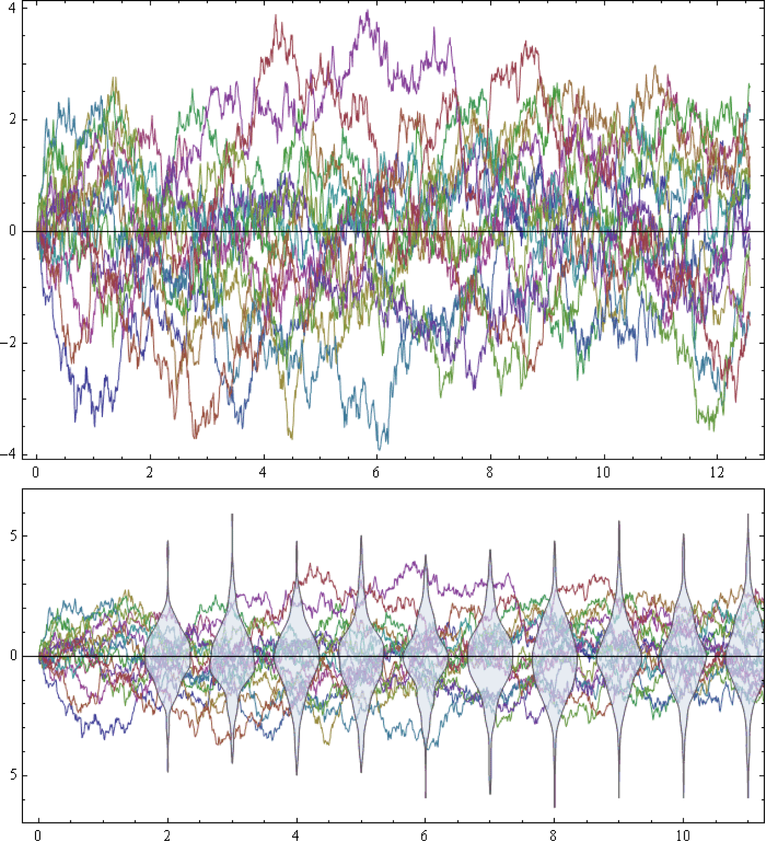
As a simple demonstration case for the statistical path-integral simulation, we have implemented the following Ito-type SDE with the nonlinear drift: f(X_t, t) and the vector Wiener process $g(X_t,t)={\displaystyle \sum {}_i}{g}_i(X_t,t)d{W}_{i,t}$, which includes plane waves (sine and cosine), as well as soliton-type sech waves and shock-wave-type tanh waves (see Figure 2). Thus:

$$d{X}_t=f(X_{t,}t)dt+{\displaystyle \sum _{i=1}^4{g}_i(X_{t,}t)d{W}_{i,t}},$$

where:

$$\begin{array}{l}\begin{array}{ccc}f(X_t,t)=-\frac{X_t}{\sqrt{X_t^2+1}},& g_1(X_t,t)=\sin (X_t),& g_2(X_t,t)=\cos (X_t),\end{array}\\ \begin{array}{cc}{g}_3(X_t,t)=\text{sech}{(0.5X}_t),& g_4(X_t,t)=\text{tanh}(0{.5X}_t)\end{array}.\end{array}$$

6. Conclusions

In this paper we have presented several different, but complimentary, modelling and computational views of controlled entropic self-organization (CESO). Motivated by the notion of perceptual error from perceptual control theory (PCT) in the setting of group decision making, we have proposed several modelling and simulation frameworks aimed at illuminating controlled self-organization phenomena: (i) a physical view of partition functions and path integrals, as well as entropy and phase transitions; (ii) a global view of functional compositions and commutative diagrams; (iii) a local view of the Kähler–Ricci flow and time-evolution of entropic action; and, finally, (iv) a computational view of various path-integral approximations.

Note that we do not intend these views of CESO to constitute any kind of normative ideal; our underlying formulation of group decision-making according to the PCT hypothesis, that actors make choices, so as to minimize their perceptual error, is merely a modelling construct, not necessarily an accurate representation of human behavior. Yet, we maintain that this construct, embodied in our four formal frameworks, provides powerful new formal tools and the basis for new empirical insights, thereby laying the foundation for other CESO models in our ongoing and future research.

References

- Powers, W.T. Feedback: Beyond behaviorism. Science 1973, 179, 351–356. [Google Scholar]
- Powers, W.T. Behaviorism and feedback control. Science 1973, 181, 1118–1120. [Google Scholar]
- Ivancevic, V.; Reid, D.; Aidman, E. Crowd behavior dynamics: Entropic path-integral model. Nonlinear Dyn 2010, 59, 351–373. [Google Scholar]
- Moussouris, J. Gibbs and Markov random systems with constraints. J. Stat. Phys 1974, 10, 11–33. [Google Scholar]
- Landau, L.D.; Lifshitz, E.M. Statistical Physics, 3rd ed; Butterworth–Heinemann: Oxford, UK, 1996. [Google Scholar]
- Hopfield, J.J. Neural networks and physical systems with emergent collective computational abilities. Proc. Natl. Acad. Sci. USA 1982, 79, 2554–2558. [Google Scholar]
- McCullough, W.S.; Pitts, W.H. A logical calculus of the ideas immanent in nervous activity. Bull. Math. Biophys 1943, 5, 115–133. [Google Scholar]
- Ivancevic, V.; Ivancevic, T. Complex Nonlinearity: Chaos, Phase Transitions, Topology Change and Path Integrals; Springer: Berlin, Germany, 2008. [Google Scholar]
- Nicolis, G.; Prigogine, I. Self–Organization in Nonequilibrium Systems: From Dissipative Structures to Order through Fluctuations; Wiley: New York, 1977. [Google Scholar]
- Ivancevic, V.; Ivancevic, T. Neuro–Fuzzy Associative Machinery for Comprehensive Brain and Cognition Modelling; Springer: Berlin, Germany, 2007. [Google Scholar]
- Tian, G.; Zhang, Z. Regularity of Kähler-Ricci flows on Fano manifolds 2013, arXiv, math.DG/1310.5897.
- Cao, H.D. Deformation of Kähler metrics to Kähler-Einstein metrics on compact Kähler manifolds. Invent. Math 1985, 81, 359–372. [Google Scholar]
- Morgan, J.W.; Tian, G. Ricci Flow and the Poincaré Conjecture. Clay Math. Monogr 2007, arXiv, math/0607607. [Google Scholar]
- Perelman, G. The entropy formula for the Ricci flow and its geometric applications 2002, arXiv.
- Rothaus, O. Logarithmic Sobolev inequality and the spectrum of Schrödinger operators. J. Funct. Anal 1981, 42, 110–120. [Google Scholar]
- Ivancevic, V.; Ivancevic, T. Quantum Neural Computation; Springer: Berlin, Germany, 2009. [Google Scholar]
- Metropolis, N.; Rosenbluth, A.; Rosenbluth, M.; Teller, A.; Teller, E. Equation of state calculations by fast computing machines. J. Chem. Phys 1953, 21, 1087. [Google Scholar]
- Feynman, R.P. Space–time approach to nonrelativistic quantum mechanics. Rev. Mod. Phys 1948, 20, 367–387. [Google Scholar]
- Ivancevic, V.; Reid, D. Turbulence and shock-waves in crowd dynamics. Nonlinear Dyn 2012, 68, 285–304. [Google Scholar]
© 2014 by the authors; licensee MDPI, Basel, Switzerland This article is an open access article distributed under the terms and conditions of the Creative Commons Attribution license (http://creativecommons.org/licenses/by/3.0/).
Share and Cite
Ivancevic, V.; Reid, D.; Scholz, J. Action-Amplitude Approach to Controlled Entropic Self-Organization. Entropy 2014, 16, 2699-2712. https://doi.org/10.3390/e16052699
Ivancevic V, Reid D, Scholz J. Action-Amplitude Approach to Controlled Entropic Self-Organization. Entropy. 2014; 16(5):2699-2712. https://doi.org/10.3390/e16052699
Chicago/Turabian StyleIvancevic, Vladimir, Darryn Reid, and Jason Scholz. 2014. "Action-Amplitude Approach to Controlled Entropic Self-Organization" Entropy 16, no. 5: 2699-2712. https://doi.org/10.3390/e16052699