Article

An Evolutionary Algorithm for the Texture Analysis of Cubic System Materials Derived by the Maximum Entropy Principle

1
School of Materials Science and Engineering, Shenyang Aerospace University, Shenyang 110136, China
2
School of Information Science and Engineering, Northeastern University, Shenyang 110189, China
3
School of Materials and Metallurgy, Northeastern University, Shenyang 110189, China
*
Author to whom correspondence should be addressed.
Entropy 2014, 16(12), 6477-6496; https://doi.org/10.3390/e16126477
Submission received: 25 July 2014 / Revised: 15 October 2014 / Accepted: 12 November 2014 / Published: 9 December 2014

Abstract

:
Based on the principle of maximum entropy method (MEM) for quantitative texture analysis, the differential evolution (DE) algorithm was effectively introduced. Using a DE-optimized algorithm with a faster but more stable convergence rate of iteration, more reliable complete orientation distribution functions (C-ODF) have been obtained for deep-drawn IF steel sheets and the recrystallized aluminum foils after cold-rolling, which are both designated as the macroscopic cubic-orthogonal symmetry. With special reference to the data processing, no more other assumptions are required for DE-optimized MEM except that the system entropy approaches the maximum.

1. Introduction

With regard to the quantitative analysis of textured materials, when the representation method for orientation distribution function (ODF) appeared primarily in an approximation, it was defined as the series of a reduced ODF (R-ODF) for crystalline grain clusters [15]; furthermore, the complete orientation distribution (C-ODF) also evolved with the development of quantitative texture analysis through several specific mathematical treatment procedures [69]. Among the different methods currently utilized, the maximum entropy method (MEM) established in keeping with the principle of maximum entropy has become the most accessible technique for the resolving of C-ODF based on a nonlinear parametric system, which was proposed independently by Wang et al. and Schaeben in the late 1980s [811]. However, during the calculation process, a massive system of nonlinear equations must be solved to reach the genuine solution. Moreover, for all the conventional algorithms for solving the nonlinear equations based on the system of analytical mathematics, a set of specific initial solutions should be selected or defined. If the designation on initial solution is not appropriate, it usually results in the iterative failure of the whole calculation process. That’s exactly what makes MEM a difficult approach to the genuine solution by means of conventional iterative algorithms [1216].
In recent years, the maximum entropy principle has been used in a wider range of applications for dealing with complex systems consisting of nonlinear variables [1721]. It is crucial for such an analytical method to solve the fuctional relevancy among multivariate nonlinear variables by means of the most accessible variables that are linearly independent of each other [2229]. In order to improve the efficiency for solving this problem, a DE algorithm was introduced for the solution procedure. The DE algorithm is a newly developed meta-heuristic approach that mainly has three advantages: detecting the true global minimum regardless of the initial parameter values, fast convergence, and the use of few control parameters. The DE algorithm is a population-based algorithm like genetic algorithms using similar operators: crossover, mutation and selection [3035]. It works to prevent the solving procedure from obscure selection of the initial solution.

2. General Principle Description

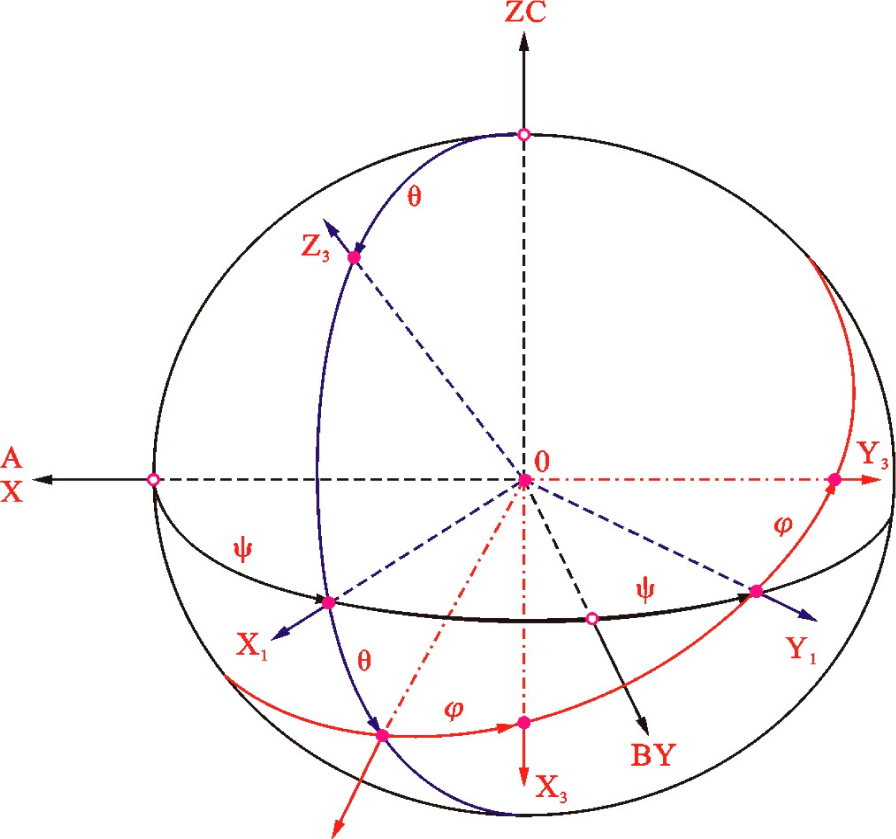
2.1. ODF Representation Derived by MEM

As with the implementation of MEM, sub-orientation space without symmetry is presented in response to the crystalline structure and texture symmetry of different materials, and then, divided into equivalent orientation units whose total number is J. Vj is defined as the volume percentage of crystalline orientation that falls coincidently in orientation unit j of the detected sample; ω (θj, ψj, φj) denotes the relative orientation density of unit j identified (θj, ψj, φj are the central Euler angles of j):
V j = ω ( θ j , ψ j , φ j ) sin θ j Δ θ Δ ψ Δ φ , j = 1 , 2 , , J
j = 1 J V j = 1
In the R-ODF series, the coefficient of the lmn th item, Wlmn, is substituted by Wr in subscript label, then, r = 1, 2, …, R; the value of R is determined by lmn where the expanded series is truncated. According to series expansion method [2,3], there should exist:
W r = j = 1 J V j R r j , r = 1 , 2 , , R
In the Equation (3), the coefficient of ODF series Wr can be calculated from experimental data. The coefficient Arj is an identified value in the case of complete macroscopic symmetry. The deduction process is elucidated in the Equation (4) as follows:
A r j = 1 3 { [ Z m n ( cos θ j ) cos ( m ψ j + n φ j ) + ( 1 ) + m Z m n ¯ ( cos θ j ) cos ( m ψ j n φ j ) ] + [ Z m n ( cos θ 2 ) cos ( m ψ 2 + n φ 2 ) + ( 1 ) + m Z m n ¯ ( cos θ 2 ) cos ( m ψ 2 n φ 2 ) ] + [ Z m n ( cos θ 3 ) cos ( m ψ 3 + n φ 3 ) + ( 1 ) + m Z m n ¯ ( cos θ 3 ) cos ( m ψ 3 n φ 3 ) ] }
In Equation (4)Zlmn(θ) denotes the augmented Jacobi polynomials; and two sets of Euler angles with the subscripts of 2 or 3 are derived from {θj, ψj, ϕj} due to the tri-fold symmetry in crystalline structure, whose values can be determined according to the reference [13,16].
In accordance with the principle of entropy maximum, there should be:
V j = e ( 1 x 0 r = 1 R x r A r j ) ; r = 1 , 2 , , R ; j = 1 , 2 , , J
In Equation (5), x (x0, x1, x2, …, xR) are the undetermined Lagrange multipliers. When Equation (5) is substituted into both Equations (2) and (3), a set of nonlinear equations on solving different x whose total number is (R + 1) are obtained:
{ j = 1 J e ( 1 x 0 r = 1 R x r A r j ) = 1 j = 1 J e ( 1 x 0 r = 1 R x r A r j ) A r j = W r
Based on the theorem that the number of unknown variables equals the amount of equations, Equation (6) is. However, it holds a set of nonlinear equations with the unknown variables sitting on their perch among the exponential terms, so it is practically infeasible to solve such a system of equations by the regular mathematical method. For this purpose, the objective function S is established for the DE algorithm.
The objective function of S, which is composed by the nonlinear equation set, can be expressed as:
Min S = ( 1 j = 1 J e ( 1 x 0 r = 1 R x r A r j ) ) 2 + r = 1 R f r ( W r j = 1 J A r j e ( 1 x 0 r = 1 R x r A rj ) ) 2
where fr ∊(0,1] is a positive parameter for controlling the effect of Wr on S, whose value should be assumed as less than 1. When Equations (6) and (7) are both substituted into DE, the values of x0, x1, x2, , xR can be solved. Then, after being substituted back to Equations (5) and (1), the complete ODF (C-ODF) can be obtained.

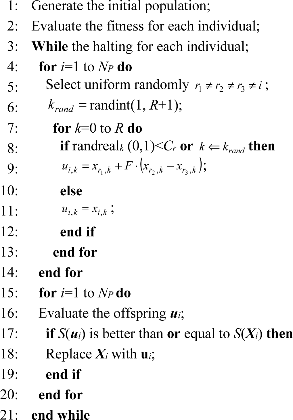
2.2. Differential Evolution Algorithm

Differential evolution (DE) is an algorithm based upon swarm evolution, which is characterized by memorizing the individual optima and sharing information in the swarm. It performs according to the mechanism of cooperation and competition among the individuals to achieve the solution of an optimization problem.
As a classic formulation, DE begins with a randomly initiated swarm population of NP in the whole accessible solution space, which is designated as X 0 = { x 1 0 , x 2 0 , , x N p 0 }, Np denotes the swarm population; furthermore, an individual with D-dimensional parameter vectors represents the initial solution of the specified problem, which is designated as x i 0 = [ x i 1 0 , x i 2 0 , , x i D 0 ], i = 1, 2, …, Np. D is the dimensionality of the optimization problem.
In this paper, S(X) is defined as the objective function to be optimized for solving the MEM nonlinear equation set, and X (x0, x1, x2, , xR) is the decision vector consisting of R + 1 variables and designated as components for the equation set to be solved, i.e., X is the solution vector and in addition termed as an individual that consists of an R + 1 dimensional parameter vector. DE algorithm executes to evolve a population including NP individuals in number, i.e., Xik =(xi0,xi1,xi2xiR) ∊ S(X), i=1,2⋯Np. So, the amount of candidate solutions is NP. x i , k G signifies the kth parameter of the ith solution vector. G denotes the Gth generation of evolution. NP doesn’t change during the evolution process once determined.
The essential feature for DE is an iterative algorithm for generating trial vectors. Mutation and crossover operators are used to generate trial vectors, and the selection operator then determines which of the vectors will survive into the next generation [3136]. In this paper, we adopt the fundamental scheme whose notation is described as “DE/rand/1/bin” strategy for solving ODF utilizing a set of experimental information [26].

2.2.1. Initialization

DE operates in a straight parallel search method. An initial population begins randomly with a uniform distribution in the whole accessible search space to activate the iterative scheme of DE. When G = 0, it starts as a population of NP parameter vectors in the R + 1 dimensionality, i.e., X ( 0 ) = { x 1 0 , x 2 0 , ... , x N P 0 }, and x i 0 = [ x i , 0 0 , x i , 1 0 , , x i , R 0 ].

2.2.2. Mutation

DE mutates and recombines the population to produce a population of NP mutant vectors, V i G = ( ν i , 0 G , ν i , 1 G , ν i , 2 G , , ν i , R G ). For each target vector x i , k G, a mutant vector ν i , k G is generated according to the following:
ν i , k G = x r 1 , k G + F ( x r 2 , k G x r 3 , k G ) , k = 0 , 1 , 2 , , R
In Equation (8)F is commonly known as a scale factor and is a positive real number. It controls the amplification of the different vector ( x r 2 , k G x r 3 , k G ). According to [10], the range of F varies within [0,2]; Three individuals, x r 1 , k G, x r 2 , k G and x r 3 , k G, are selected randomly from the current population, where the indices r1, r2 and r3 represent the random and mutually different integers generated within the range of [1,NP] so that r1,r2,r3∊{1,2,…Np}, and furthermore different from index i such that r1r2r3i. It should be noted that these indices must be different from each other and out of the proceeding index labeled with i so that Np should be ≥ 4. If one component of the mutant vector overflows the search space, then a new substitute value is generated by activating initialization.

2.2.3. Crossover

The target vector is mixed with the mutated vector, utilizing that the parent vector is discretely recombined with the mutated vector to yield a trial vector, U i G = ( u i , 0 G , u i , 1 G , u i , 2 G , , u i , R G ) so as to balance the differential mutation search strategy:
u i , k G = { v i , k G , r a n d ( i , k ) C r o r k = k r a n d , x i , k G , r a n d ( i , k ) > C r o r k k r a n d
In Equation (9), rand(i, k) ∊ [0,1] is a uniformly generated random number ranging within [0,1]. i=1,2,…,Np and k = 0,1,2,…,R refers to the kth parameter of the ith vector, which performs to establish a u i , k G through discrete recombination. k r a n d { 0 , 1 , 2 , ... , R } denotes a randomly triggered integer index, which ensures that u i , k G acquires at least one mutant vector different from v i , k G; otherwise, no new parent individual would be generated and the population should still remain unchanged. Cr ∊ [0,1] is the crossover probability constant, which is empirically calibrated by the user.

2.2.4. Selection

A greedy criterion is adopted for DE to decide whether or not the trial vector u i , k G should become a member generation of G + 1 after it is compared to the target vector x i , k G. Only when the u i , k G yields a better fitness function value than the x i , k G does can it be set to x i G + 1. Otherwise, the previous target vector x i , k G becomes retained. The selection scheme is described as follows for an issue on minimization:
x i , k G + 1 = { u i , k G , S ( u i , k G ) < S ( x i , k G ) , x i , k G , S ( u i , k G ) S ( x i , k G ) .
A typical pseudo-code of DE algorithm according to the “DE/rand/1/bin” mutation scheme [1113] is described in Algorithm 1 as follows:
Algorithm 1. Pseudo-code flowchart of a typical DE algorithm with “DE/rand/1/bin” mutation scheme
Entropy 16 06477f5
The number of control parameters in DE is very small. The classic DE has three parameters that need to be adjusted: (a) the population size NP; (b) the mutation scale factor F∊ [0,2]; (c) the crossover rate Cr∊[0,1]. How these parameters affect the performance of DE algorithm is well discussed in the references [3034]. As for the termination conditions, either a maximum iteration number corresponding to the objective function for evaluation or a fixed tolerance on precision error of the desired solution can be proposed in advance. It can be shown that this algorithm is favorable due to its simplicity in formulation, easiness to be operated and suitability for calculation by computers.
In DE algorithm, the population size is set as NP = 300, which is determined according to the principle: 3RNP ≤ 9R, suggested by Storn and Price et al. [3336] due to the large value of R = 58, when l equals to 16; cross rate, Cr = 0.2, which is confirmed by the 59 linearly independent vectors of Xik and also referred to the suggestion by Storn and Price et al. [32,33]; the scaling factor is referred to as F = randrealj (0.2,05); the tolerance on precision error in equality is set as δ=5×10⁻⁴ according to the references proposed in [3133]. The algorithm is quite robust with respect to the algorithmic parameters F and Cr. Setting F = 0.35 and Cr = 0.2 will give generally good convergence on a wide range of problems according to references [3440].
The calculated results should be adjusted in terms of normalization for comparison with each other. For this purpose, in the whole programming procedure of solving genuine C-ODF, the parameter settings are fixed as the followings unless a change is mentioned: In MEM, for simplicity, all of fr (r = 1, 2, 3, …, R) in the proposed objective function S(X) are suggested to perform as a constant of 1/16 experientially since that the truncation point was set to l = 16. Since that the DE optimized MEM is designated for the quantitative texture analysis on the cubic materials with macro symmetric texture, therefore, the total amount of orientation units corresponding to sub-space is set to 1296 (72 × 18), i.e., J = 1296.

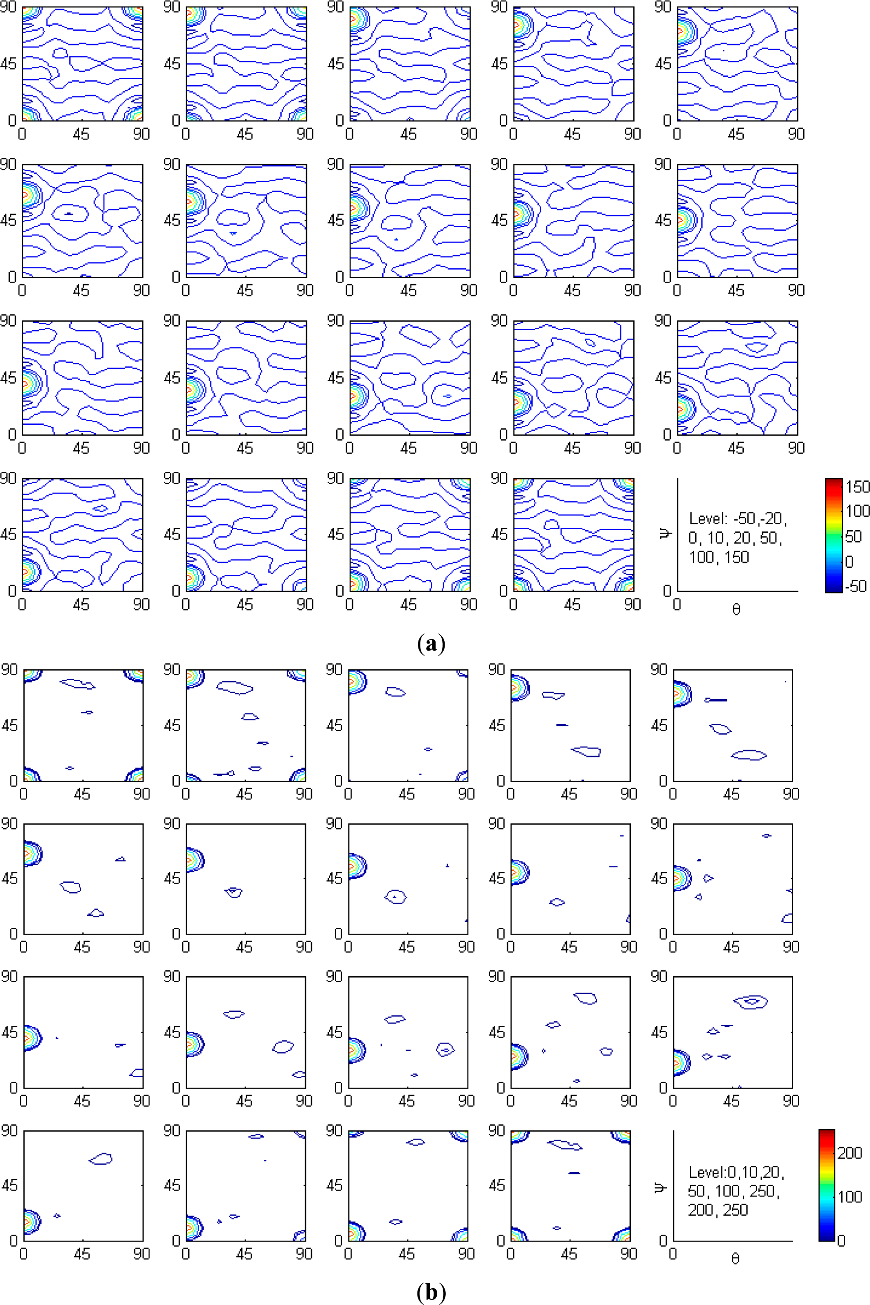
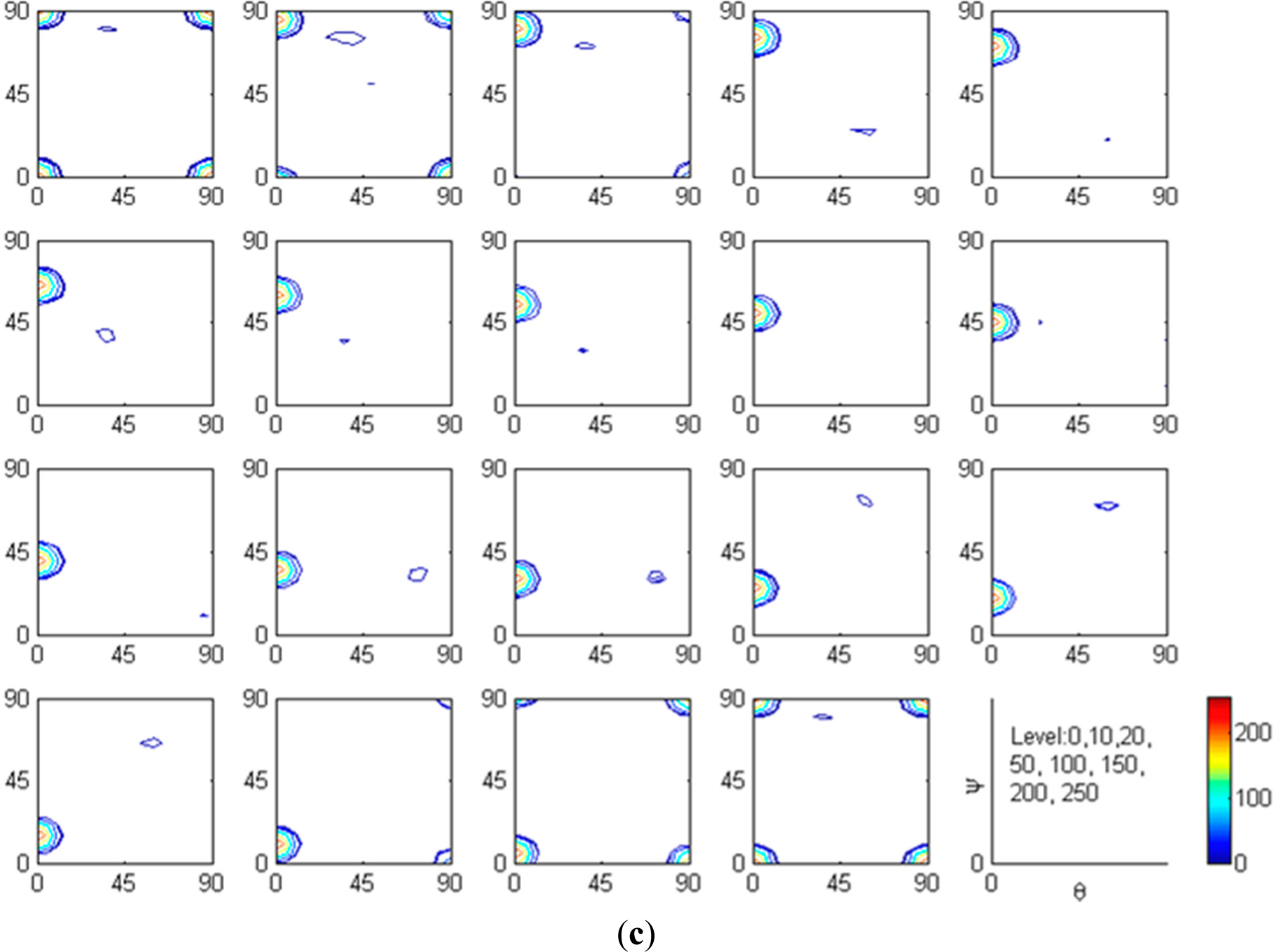
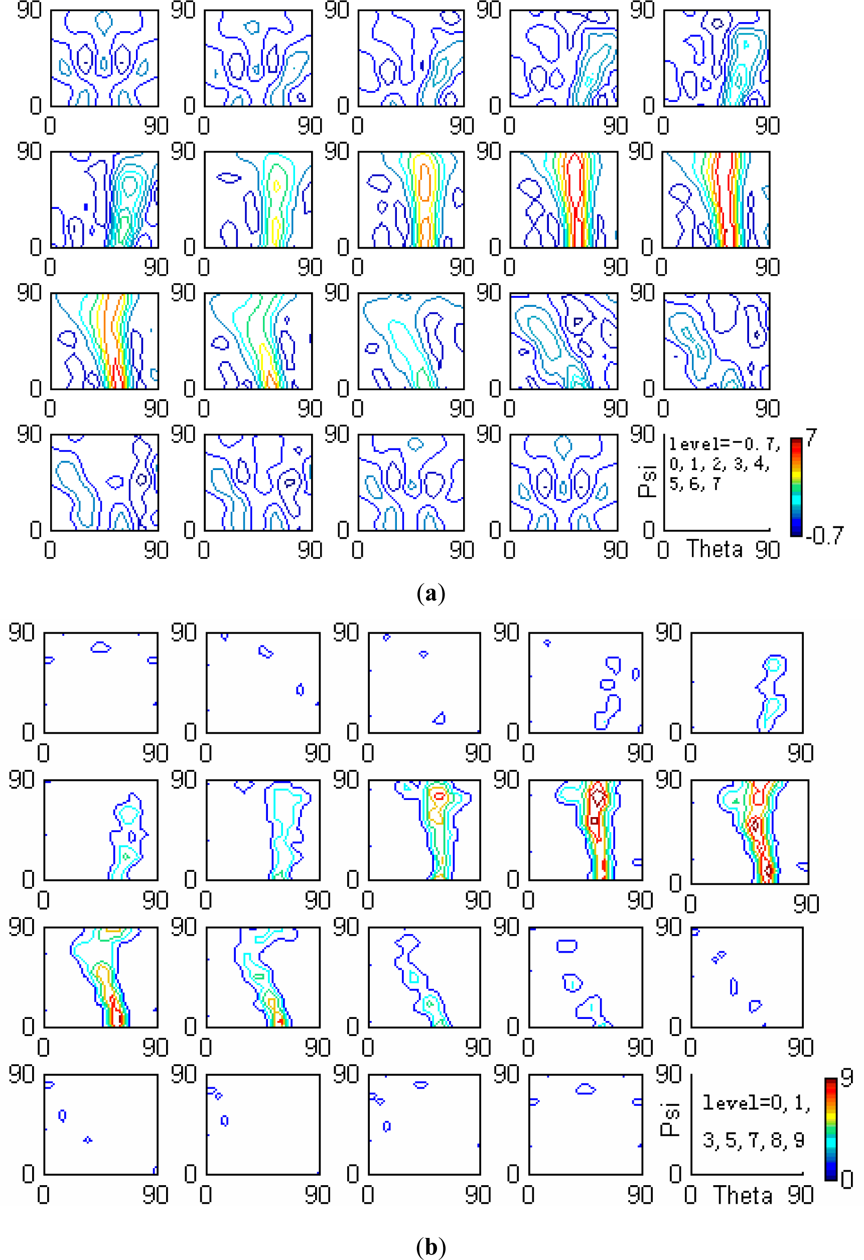
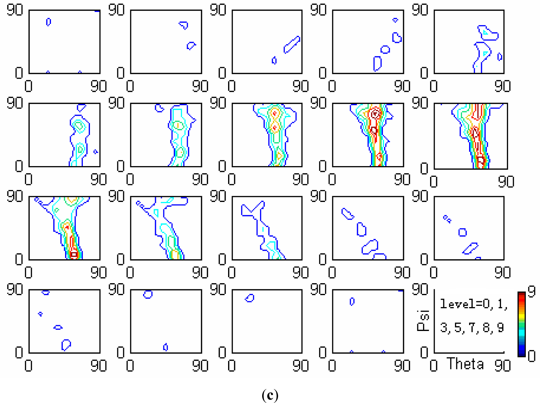
3. Experimental Results and Discussion

The test samples were the recrystallized aluminum foils after cold-rolling (fcc), and the deep-drawn IF steel sheets (bcc), respectively. More than two samples for each group in comparison were examined systematically in this work. The measurements were carried out using an X'Pert diffractometer from PANalytical (Almelo, The Netherlands) equipped with a Cobalt target (λ = 0.179 nm). Three experimental pole figures of (111), (200), and (220) corresponding to the fcc structure, and (110), (200), and (211) to the bcc structure have been measured (α = 0°~70°, β = 0°~360°, △α = △β = 5°), respectively.

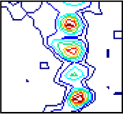
3.1. ODF Representation on Aluminum Foils

The results of ODF representation derived by different algorithms are shown in comparison as Figure 1. It can be obviously observed that the ODF representation of the fcc aluminum foil sample consists of exclusively intensive {100} <001> cubic texture. By adopting the traditional Two-step Method [6], its maximum orientation density is ωmax = 167.51, and there still exist “ghost peaks” together with negative zones in divergence shown as Figure 1a, whose negative value reaches as low as −60.16. The C-ODF derived by a damped Newtown method based on MEM is shown in Figure 1b, ωmax = 260.05. There exist no “ghost peaks” or negative areas any more. Moreover, the C-ODF derived by DE optimized MEM is shown as Figure 1c, ωmax = 265.97. It is verified that the positions of the texture components, i.e., the {ψ,θ,φ} presented in the ODF configuration are completely identical to each other except that their intensities differ more or less.
Although the value of the primary {100} <001> cubic texture component in Figure 1b appears almost identical to that in Figure 1c, it has been achieved through 4000 iterations on condition that an initial solution selection must be selected appropriately. By comparison, its magnitude is ten times larger than that derived by DE. The results calculated for the Aluminum foils corresponding to the iteration number, Gmax, are list in details in Table 1.
It is indicated from Table 1 that, when k exceeds 600, Smin converges to a convinced value. Hence, S ( u i , k 600 ) is designated as the genuine solution when Gmax equals to 600, and the C-ODF can be resolved consequently.

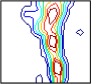
3.2. ODF Representation on IF-steel Sheets

The samples are 0.8 mm deep-drawn plates of standard IF steel provided by a commercial steel plant. More than two groups of samples were compared in practice. The results of ODF representation derived by different algorithms are compared with each other and shown in Figure 2. In R-ODF, its maximum orientation density is ωmax = 7.07, and the “ghost peaks” and dispersive negative value zones still appear, as shown in Figure 2a, whose negative value grade approaches as low as −0.69. Correspondingly, the magnitude of C-ODF derived by DE optimized MEM, shown in Figure 2c, reaches ωmax = 9.75. No “ghost peaks” or negative areas appear. The result derived by a damped Newtown method is also shown in Figure 2b. It is observed that the positions of the primary γ-fiber (<111>//ND) texture component derived by different methods are completely identical to each other in Figure 2. Therefore, it can be verified that the positions of the texture components, i.e., the {ψ,θ,φ} presented in the ODF configuration are completely identical to each other except that their intensities differ more or less. Although the value of the strongest texture component is nearly identical to that in Figure 2c, ωmax = 9.53, it has been achieved through 5000 iterations with a set of initial solution being designated appropriately. The iteration number also stands ten times greater than that derived by DE. A typical calculation result of the IF steel sheets corresponding to the iteration number, Gmax, is list in details in Table 2.
It is indicated from Table 2 that, when Gmax exceeds 500, Smin converges to a fixed value. Hence, S ( u i , k 500 ) is designated as the genuine solution when Gmax equals to 500, and the C-ODF can be resolved consequently. The φ = 45° section diagrams in Table 2 are the concise representation on bcc materials, which indicates the {111} γ-fiber texture component parallel to the rolling surface of IF steel. The diagrams illustrate the variation tendency of the primary texture component in IF steel corresponding to different iterations obviously. When Gmax stands at 500, the configuration of φ-section is nearly identical to that with 5000 iterations.
It should be noted that DE is a population-based search strategy and performs through the stochastic optimization algorithm, which differs prominently in the sense that distance and direction information from the current population are utilized to guide the search process compared with other evolutionary algorithms (EA). Consequently, the optimum solution for each different calculation under the same initial conditions doesn’t remain constant but rather varies within a very limited range. The variation is rational due to the robustness of global optimum corresponding to the prerequisite that the solution’s behavior changes continuously with the initial conditions. Since that there is no need for an initial preset solution for executing the MEM, it is a well-posed problem.
In conclusion, it is proved that DE is a more efficient algorithm for global optimization and also an evolutionary method for ODF representation of textured materials so as to make the results much more reliable with much less computation time.

4. Conclusions

In this article the differential evolution algorithm has been effectively applied for an improved ODF representation on cubic textured materials by MEM without designating a set of initial solutions.
  • The complete ODF derived by differential evolution is entirely feasible due to its simple parameterization scheme, whose primary texture component is endowed with the configuration pattern in more details with much less iteration rounds.
  • The differential evolution algorithm is suitable for solving the nonlinear equations of quantitative texture analysis, which is proposed in this article for the ODF representation on the cubic textured materials.
  • Differential evolution is characterized by global optima to provide better computation results via much less iterations in comparison with those deduced by conventional damped Newton iteration, which shows a universal optimization mechanism for quantitative texture analysis that follows the maximum entropy principle.

Acknowledgments

The authors gratefully acknowledge the National Foundation of Natural Science (No. 51171120) for the financial support. The authors also gratefully acknowledge the Fundamental Research Funds for the Central Universities (N110404024) for the financial support.

Appendix

A. Analysis of the Reduced ODF(R-ODF) via Two-step Method

In order to specify an orientation, it is necessary to set up a reference system known as a coordinate system. Two sets are required: one is related to the whole specimen, and the other is related to the crystalline coordinate. Both coordinates are Cartesian and preferably right-handed. The 0-ABC is set on the specified specimen, which signifies the same representation as a pole figure. The rolling direction (RD), transverse direction (TD) and normal direction to the rolling plane (ND) are the three ones typically defined as a geometric framework; furthermore, another Cartesian coordinate system of 0-XYZ is also set corresponding to an individual grain specified in combination with 0-ABC. As a result, the {ψ,θ,φ} of three Euler angles that are derived from the crystalline coordinate in relation to the specimen coordinate, is termed as the crystalline orientation shown as Figure 3. ω(θ,ψ,φ) is further defined as the orientation density that represents the volume fraction of grains in a orientation unit, and is described as:
ω ( θ , ψ , φ ) = K ω Δ V V sin θ Δ θ Δ ψ Δ φ
In the Equation (11), sin θΔθΔψΔφ is defined as the orientation unit incorporating the crystalline orientation of {ψ,θ,φ}; ΔV/V represents the volume fraction of grains that falls coincidently in the orientation unit, designating the occurrence probability of the above crystalline orientation to the specified orientation unit; Kω is defined as a scale factor, and if the value of ω(θ,ψ,φ) is fitted to 1 corresponding to a non-textured condition, then Kω=8π2. In this case, ω(θ,ψ,φ) is termed as the relative orientation density.
The orientation distribution function (ODF) of ω(θ,ψ,φ) can be obtained by means of various orientation measurement techniques, but the widespread applications still remain focused on calculating ODF from {hkl} pole figures measured by X-ray diffraction technology, i.e., the series expansion method (SEM). According to the principle of spherical harmonic analysis, both the pole figure of qj(α, β) and the ODF of ω(θ,ψ,φ) can be expanded into series, then:
q j ( α , β ) = = 0 m = Q m j P m ( cos α ) e i m β
In Equation (12), Q m j designates the coefficient of the ℓm th item corresponding to the jth pole figure, which can be determined by reference to Equation (13), and then calculated from each value of qj(α, β) measured experimentally:
Q m j = 1 2 π 0 2 π 0 π q j ( α , β ) P m ( cos α ) e i m β sin α d α d β
P m ( cos α ) represents the associated Legendre polynomials performing both in Equations (12) and (13); α together with β designate the polar angle and argument, respectively.
Likewise, the ODF of ω(θ,ψ,φ) is expended into series as:
ω ( θ , ψ , φ ) = = 0 m = n = W m n Z m n ( cos θ ) e i m ψ e i n φ
In Equation (14)Wℓnm designates the coefficient of the ℓnm th item corresponding to the ODF; Zℓnm(cos θ) represents the augmented Jacobi polynomials. Based upon the relationship between the two coefficients, the coefficient of ODF, i.e., Wℓnm could be calculated by reference to the Equation (15) after the designated pole figures being measured:
Q m j = 2 π ( 2 2 + 1 ) 1 / 2 n = W m n P n ( cos Θ j ) e i n Φ j
For Equation (15), Θj and Φj are defined as the polar and argument angles, respectively. Meanwhile, both angles are derived from the normal direction of a {khl} plane that lies in the crystalline coordinate system for the jth pole figure. Subsequently, the ODF can be worked out under Equation (14) again. For cubic textured materials, if the crystal symmetry and geometrical symmetry of the designated specimen are both taken into consideration, the calculation on can reach to 16 or 22 with only two complete pole figures. However, it is difficult to implement the measurement on the complete pole figure in practice; furthermore, it is more difficult to investigate the superficial orientation distribution in textured materials. It is attributed to Bunge who presented such mathematical procedures [2,3] for realizing the purpose discussed above by adopting the reflection method proposed by Schulz [41]. The Two-step Method has been widely recognized and adopted after that it was first proposed by Liang and Xu et al. in 1981 [6].
The principle goes that for the first step, the normalized factors of Nj and W0n for the pole figures should be determined primarily by computing the integral along the argument β, which is described by Equation (16):
{ j = 1 k { P n ( cos Θ j ) e i n Φ j 0 χ F q 0 j M P ( cos α ) sin α d α } N j = 0 λ n = [ 4 π 2 ( 2 2 + 1 ) 1 / 2 { j = 1 k P n ( cos Θ j ) P n ( cos Θ j ) e i ( n + n ) Φ j } × 0 χ F P ( cos α ) P ( cos α ) sin α d α ] W 0 n = 0 = 1 , 2 , , λ , n = 0 , ± 1 , ± 2 , , ± [ 0 χ F q 0 j M ( α ) } 2 sin α d α ] N j = 0 λ n = 4 π 2 ( 2 2 + 1 ) 1 / 2 × P n ( cos Θ j ) e i n Φ j 0 χ F q 0 j M ( α ) P ( cos α ) sin α d α } W 0 n = 0 j = 1 , 2 , , k
For the second step, the rest of Wℓnm should be determined by grouping the m clusters according to Equation (17):
{ = | m | λ n = [ j = 1 k 0 χ F P m ( cos α ) P m ( cos α ) sin α d α × { P n ( cos Θ j ) P n ( cos Θ j ) e i ( n + n ) Φ j } × 4 π 2 ( 2 2 + 1 ) 1 / 2 ] W m ¯ n j = 1 k P n ( cos Θ j ) e i n Φ j × 0 2 π 0 χ F q j M ( α , β ) P m ( cos α ) e i m β sin α d α d β ] N j = 0 j = 1 , 2 , , k
The ω(θ,ψ,φ) deduced from such two steps is designated as a reduced ODF(R-ODF).

B. Analysis of the Complete ODF(C-ODF) via the Maximum Entropy Method

It is generally known that the R-ODF contains some negative value areas in Euler space, which renders some “ghost peaks” that do not correspond to the authentic texture components; and even some distorted peaks in shape that really correspond to the genuine texture components. The fundamental causes are rooted in the lack of on the odd items in the expanded orientation density series complying with the Friedel law of X-ray diffraction, and furthermore in combination with the effect of truncation error, which were indicated by Matthies in 1979 [810]. The measurement and calculation on the C-ODF without containing the negative value areas after an appropriate completion for the odd items still remains as challenging as ever for researchers.
It is necessary to apply a new mathematical theory or technique to reveal the whole configuration of C-ODF, through which the most accessible results can be acquired on the premise of insufficient information. Therefore, two prerequisites must be satisfied synchronously: (a) being consistent with all known information; (b) being irrelevant to the unknown information with a maximum limit. The maximum entropy method (MEM) in conformity with the principle of maximum information entropy can meet such two prerequisites.
The MEM was first proposed by Wang and Liang [13] for investigating the crystalline orientation distribution of textured materials using an innovative information entropy theory in 1987. The independent Euler subspace without symmetry is principally divided into N = 72 equivalent orientation units [16], shown as Figure 4.
When ψ is divided by 5° from 0° to 90°, it would separate into 18 layer areas, and then the total number of orientation units divided from the whole Euler sunspace sums up to J = N × 18 = 72 × 18 = 1296 [13,16]. The Euler angle, gj = {ψj,θj,φj} at each central point of all the orientation units is set as the azimuth angle of the corresponding orientation unit; and the average density of orientation in the jth orientation unit is defined as Vj. The volume fraction of each orientation unit is set as 1/1296 corresponding to a non-textured specimen. According to the theory of R-ODF, Vj should be described by Equation (18),
V j = ω ( θ j , ψ j , φ j ) sin θ j Δ ψ Δ θ Δ φ
Moreover:
j = 1 J V j = 1
The description on system entropy is shown as Equation (20) by reference to the definition given by Jaynes in 1957 [41]:
H ( V ) = k j = 1 J V j ln V j
Equation (20) designates the magnitude of systematic uncertainty, and k denotes the scale factor whose value is usually set to 1. When the total amount of ℓmn is indicated by R, then there should exist the relation in Equation (21):
A r j = { Z m n ( cos θ j ) cos ( m ψ j + n φ j ) + ( 1 ) Z m n ( cos θ j ) cos ( m ψ j n φ j ) }
Moreover:
W r = j = 1 J A r j V j , r = 1 , 2 , 3 , , R
In Equation (22)Wr denotes the coefficient of the ODF series. Moreover, Equation (23) should be achieved according to the maximum entropy principle as follows:
H ( V 1 , V 2 , , V J ) = j = 1 J V j ln V j + λ 0 ( j = 1 J V j 1 ) + r = 1 R [ λ r ( j = 1 J ( V j A r j W r ) ]
A partial differential is performed upon the variable Vj in Equation (23), and its result is further set to 0, i.e., H V j = 0, then, there exists:
H V j = j = 1 J { [ ln V j + 1 ] + λ 0 × 1 ) + r = 1 R λ r A r j } = 0
Only on the condition that each item in the formula above equals to zero can the sum over all the partial derivatives reach to naught, if any. Then:
{ ln V j + 1 + λ 0 + r = 1 R λ r A r j } = 0
As a result, Vj is further concluded as Equation (26):
V j = exp ( 1 λ 0 r = 1 R λ r A r j )
A group of nonlinear equation sets, shown as the Equation (27), can be formulated by substituting the Equation (26) into the Equations (19) and (22), respectively:
{ j = 1 J e ( 1 λ 0 r = 1 R λ r A r j ) = 1 r = 1 R A r j e ( 1 λ 0 r = 1 R λ r A r j ) = W r
According to the principle of solving the equation sets, only when the number of unknown variables equals the amount of equations can they be solvable. However, Equation (27) consists of a system of nonlinear equations with the unknown variables sitting in the position of the exponential terms; therefore, it is nearly infeasible to be solved by the regular mathematical methods. Up to now, researchers still make unceasing progress in exploring the possible paths for resolving the problem of MEM [4244].
Conservatively, a set of λ0, λ1, λ2,…, λR can be solved by the damped Newton method or the steepest descent method, and furthermore substituted back into Equation (26), then all of Vj can be determined. After Vj is substituted back into Equation (18) and further transformed to Equation (28), the C-ODF of ω(θj,ψj,φj) can be resolved from the Equation (28), in the same expression as the Equation (1).
ω ( θ j , ψ j , φ j ) = V j / sin θ j Δ θ j Δ ψ j Δ φ j

Author Contributions

Dapeng Wang conceived, designed, and performed the study. Dapeng Wang and Dazhi Wang computed and analysed the experimental data in the paper. Dapeng Wang, Baolin Wu, Fu Wang and Zhide Liang wrote and revised the paper together. All of the authors shared the idea, data analysis, numerical results and presentation of the paper. All of the five authors have discussed, read and approved the final manuscript.

Conflicts of Interest

The authors declare no conflict of interest.

References

  1. Harris, G.B. Quantitative measurement of preferred orientation in rolled Uranium. Philos. Mag 1952, 43, 113–123. [Google Scholar]
  2. Bunge, H.J. Mathematische Methoden der Texturanalyse; Akademie-Verlag: Berlin, Germany, 1969; pp. 36–52. [Google Scholar]
  3. Bunge, H.J. Texture Analysis in Materials Science; Buttleworths: London, UK, 1982; pp. 102–165. [Google Scholar]
  4. Heizmann, J.J.; Laruelle, C. Simultaneous measurement of several X-ray pole figures. J. Appl. Cryst 1986, 19, 467–472. [Google Scholar]
  5. Kock, U.F.; Tome, C.N.; Wenk, H.R. Texture and Anisotropy: Preferred Orientation in Polycrystals and Their Effect on Materials Properties, 2nd ed.; Cambridge University Press: Cambridge, UK, 2005; pp. 36–58. [Google Scholar]
  6. Liang, Z.; Xu, J.; Wang, F. Three Dimensional Orientation Analysis on Textured Materials—ODF Analysis; Northeastern University of Technology Press: Shenyang, China, 1986; pp. 80–116. [Google Scholar]
  7. Roe, R.J.; Krigbaum, W.R. Description of crystallite orientation in polycrystal materials III. General solution to pole figure inversion. J. Appl. Phys 1965, 36, 2024–2031. [Google Scholar]
  8. Matthies, S. Reproducibility of the orientation distribution function of texture samples from pole figures (ghost phenomena). Phys. Status Solidi B 1979, 92, 135–138. [Google Scholar]
  9. Matthies, S.; Vinel, G.W. On the reproduction of the orientation distribution function of texturized samples from reduced pole figures using the conception of a conditional ghost correction. Phys. Status Solidi B 1982, 112, 111–114. [Google Scholar]
  10. Matthies, S.; Wenk, H.R. ODF reproduction with conditional ghost correction. In Preferred Orientation in Deformed Metals and Rocks: An Introduction to Modern Texture Analysis; Wenk, H.R., Ed.; Academic Press Inc: New York, NY, USA, 1985; pp. 139–147. [Google Scholar]
  11. Matthies, S.; Wenk, H.R.; Vinel, G.W. Some basic concepts of texture analysis and comparison of three methods to calculate orientation distributions from pole figures. J. Appl. Crystallogr 1988, 21, 285–304. [Google Scholar]
  12. Schaeben, H. Entropy optimization in quantitative texture analysis. J. Appl. Phys 1988, 64, 2236–2237. [Google Scholar]
  13. Wang, F.; Xu, J.; Liang, Z. Inverse pole figure determination according to the maximum entropy method. Proceedings of Textures of Materials ICOTOM-8: The Eighth International Conference on Textures of Materials, Santa Fe, NM, USA; 1987. [Google Scholar]Kallend, J.S.; Cottstein, G. (Eds.) The Metallurgical Society; Warrendale, PA, USA, 1988; pp. 111–114.
  14. Wang, F.; Xu, J.; Liang, Z. Determination of the ODF of hexagonal symmetry materials according to the maximum entropy method. Textures Microstruct 1989, 10, 217–226. [Google Scholar]
  15. Wang, F.; Xu, J.; Liang, Z. Application of maximum entropy method to the inverse pole figure determination of cubic materials. J. Appl. Cryst 1991, 24, 126–128. [Google Scholar]
  16. Wang, F.; Xu, J.; Liang, Z. Determination of the cubic system materials by the maximum-entropy method. Textures Microstruct 1992, 19, 55–58. [Google Scholar]
  17. McIntyre, N.S.; Pratt, A.R.; Piao, H.; Maybury, D.; Splinter, S.J. Resolution enhancement of X-ray photoelectron spectra by maximum entropy de-convolution. Appl. Surf. Sci 1999, 144, 156–160. [Google Scholar]
  18. Martyushev, L.M.; Seleznev, V.D. Maximum entropy production principle in physics, chemistry and biology. Phys. Rep 2006, 426, 1–45. [Google Scholar]
  19. Sankaran, S.; Zabaras, N. A maximum entropy approach for property prediction of random microstructures. Acta Mater 2006, 54, 2265–2276. [Google Scholar]
  20. Abramov, R.V. An improved algorithm for the multidimensional moment-constrained maximum entropy problem. J. Comput. Phys 2007, 226, 621–644. [Google Scholar]
  21. Li, H.S. Maximum entropy method for probabilistic bearing strength prediction of pin joints in composite laminates. Compos. Struct 2013, 106, 626–634. [Google Scholar]
  22. Wang, H.; Liu, F.; Ehlen, G.J.; Herlach, D.M. Application of the maximal entropy production principle to rapid solidification: A multi-phase-field model. Acta Mater 2013, 61, 2617–2627. [Google Scholar]
  23. Tseng, C.Y.; Tuszynski, J. Maximum entropy in drug discovery. Entropy 2014, 16, 3754–3768. [Google Scholar]
  24. Harte, J.; Newman, E.A. Maximum information entropy: A foundation for ecological theory. Trends Ecol. Evol 2014, 29, 384–389. [Google Scholar]
  25. Martyushev, L.M.; Seleznev, V.D. The restrictions of the maximum entropy production principle. Physica A 2014, 410, 17–21. [Google Scholar]
  26. Harremoës, P.; Topsøe, F. Maximum entropy fundamentals. Entropy 2001, 3, 191–226. [Google Scholar]
  27. Puig, B.; Akian, J.L. Non-Gaussian simulation using Hermite polynomials expansion and maximum entropy principle. Probab. Eng. Mech 2004, 19, 293–305. [Google Scholar]
  28. Zhao, Q.; Kurata, H. Use of maximum entropy principle with Lagrange multipliers extends the feasibility of elementary mode analysis. J. Biosci. Bioeng 2010, 110, 254–261. [Google Scholar]
  29. Guo, C.; Li, F. An improved algorithm for support vector clustering based on maximum entropy principle and kernel matrix. Expert Syst. Appl 2011, 38, 8138–8143. [Google Scholar]
  30. Fogel, D.B. Evolutionary Computation: Toward a New Philosophy of Machine Intelligence, 3rd ed.; IEEE Press: New York, NY, USA, 2006; pp. 34–65. [Google Scholar]
  31. Hrstka, O.; Kucerova, A. Improvements of real coded genetic algorithms based on differential operators preventing premature convergence. Adv. Eng. Softw 2004, 35, 237–246. [Google Scholar]
  32. Rainer, S.; Price, K. Differential evolution—A simple and efficient heuristic for global optimization over continuous spaces. J. Glob. Optim 1997, 11, 341–359. [Google Scholar]
  33. Price, K.; Storn, R.; Lampinen, J. Differential Evolution—A Practical Approach to Global Optimization; Springer-Verlag: Berlin, Germany, 2005; pp. 19–45. [Google Scholar]
  34. Ali, M.M.; Torn, A. Population-set based global optimization algorithms: Some modifications and numerical studies. Comput. Oper. Res 2004, 10, 1703–1725. [Google Scholar]
  35. Kaelo, P.; Ali, M.M. A numerical study of some modified differential evolution algorithms. Eur. J. Oper. Res 2006, 169, 1176–1184. [Google Scholar]
  36. Bergey, P.K.; Ragsdale, C. Modified differential evolution: A greedy random strategy for genetic recombination. Omega 2005, 33, 255–265. [Google Scholar]
  37. Back, T.; Schwefel, H.P. An overview of evolutionary algorithms for parameter optimization. Evol. Comput 1993, 1, 1–23. [Google Scholar]
  38. Yao, X.; Liu, Y.; Lin, G. Evolutionary programming made faster. IEEE Trans. Evol. Comput 1999, 3, 82–102. [Google Scholar]
  39. Storn, R. System design by constraint adaptation and differential evolution. IEEE Trans. Evol. Comput 1999, 3, 22–34. [Google Scholar]
  40. Liang, K.H.; Yao, X.; Newton, C.S. Adapting self-adaptive parameters in evolutionary algorithms. Appl. Intell 2001, 15, 171–180. [Google Scholar]
  41. Jaynes, E.T. Information theory and statistical mechanics. Phys. Rev. Lett 1957, 106, 620–630. [Google Scholar]
  42. Böhlke, T. Application of the maximum entropy method in texture analysis. Comput. Mater. Sci 2005, 32, 276–283. [Google Scholar]
  43. Böhlke, T. Texture simulation based on tensorial Fourier coefficients. Comput. Struct 2006, 84, 1086–1094. [Google Scholar]
  44. Junk, M.; Budday, J.; Böhlke, T. On the solvability of maximum entropy moment problems in texture analysis. Math. Models Methods Appl. Sci 2012, 22. [Google Scholar] [CrossRef]
Figure 1. Constant-φ section of ODF representation for a Aluminum foil in comparison derived by different algorithms. (a) R-ODF derived by Two-step Method; (b) C-ODF derived by MEM using the damped Newton algorithm, G = 4000 iterations; (c) C-ODF derived by MEM using DE algorithm, G = 600.
Entropy 16 06477f1Entropy 16 06477f1a
Figure 2. Constant-φ section of ODF representation for IF steel sheet in comparison derived by different algorithms. (a) R-ODF derived by Two-step Method; (b) C-ODF derived by MEM using the damped Newton algorithm, Gmax = 5000 iterations; (c) C-ODF derived by MEM using DE algorithm, Gmax = 500.
Entropy 16 06477f2Entropy 16 06477f2a
Figure 3. The rectangular coordinate system of a specimen in combination with a crystalline one.
Entropy 16 06477f3
Figure 4. The division of 72 equivalent orientation units.
Entropy 16 06477f4
Table 1. The effect of iteration number on the calculation results of Al foils using DE optimized MEM.
GmaxMaximum iteration number
5010020060010004000
Objective values, Smin5.19 × 10−22.09 × 10−21.76 × 10−34.91 × 10−41.05 × 10−47.62 × 10⁻⁵
CPU time, t (s)3.2056.79512.89529.94063.245234.125
ωmax283.07281.95263.50265.97264.96265.95
Table 2. The effect of iteration number on the calculation results of IF steel using DE optimized MEM.
GmaxMaximum iteration number
5010020050010005000
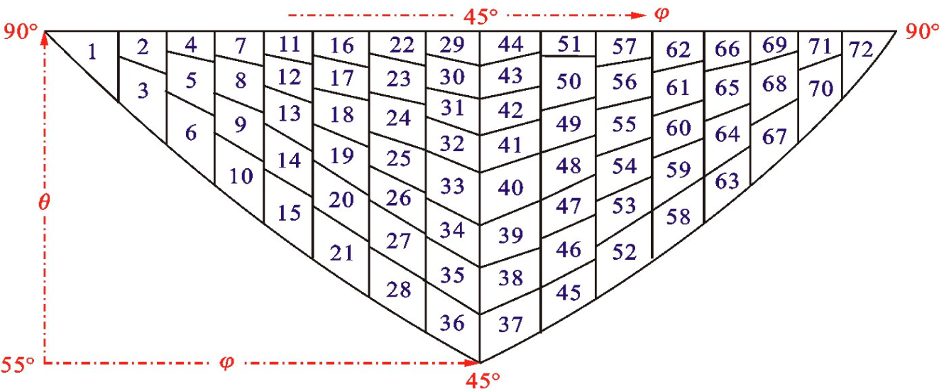
φ = 45° section in details
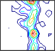
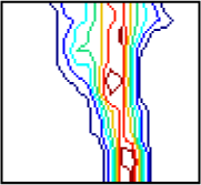
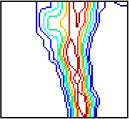
Entropy 16 06477f6Entropy 16 06477f7Entropy 16 06477f8Entropy 16 06477f9Entropy 16 06477f10Entropy 16 06477f11
Objective values, Smin5.19 × 10−22.09 × 10−23.76 × 10−34.97 × 10−41.35 × 10−43.94 × 10⁻⁵
CPU time(s)3.2056.79512.89529.94083.765312.350
ωmax11.3611.0410.429.759.8110.03

