Plant Friendly Input Design for Parameter Estimation in an Inertial System with Respect to D-Efficiency Constraints

Abstract

System identification, in practice, is carried out by perturbing processes or plants under operation. That is why in many industrial applications a plant-friendly input signal would be preferred for system identification. The goal of the study is to design the optimal input signal which is then employed in the identification experiment and to examine the relationships between the index of friendliness of this input signal and the accuracy of parameter estimation when the measured output signal is significantly affected by noise. In this case, the objective function was formulated through maximisation of the Fisher information matrix determinant (D-optimality) expressed in conventional Bolza form. As setting such conditions of the identification experiment we can only talk about the D-suboptimality, we quantify the plant trajectories using the D-efficiency measure. An additional constraint, imposed on D-efficiency of the solution, should allow one to attain the most adequate information content from the plant which operating point is perturbed in the least invasive (most friendly) way. A simple numerical example, which clearly demonstrates the idea presented in the paper, is included and discussed.

1. Introduction

The choice of an input signal used for actuation of the system is critical in the task of model building and parameter identification. System identification is the process of constructing an accurate and reliable dynamic mathematical model of a system from observed data and available knowledge. It is a common practice to perturb the system of interest and use the resulting data to build the model [1–3]. The accuracy of parameter estimates is increased by the use of optimal excitation signals [4,5]. The pertinence of a model is the critical factor for proper tuning of a controller, usually performed as a model-based optimisation task. An inaccurate model can significantly influence the performance of the control loop, and finally deteriorate the quality of the plant product. The control performance assessment has a large impact on the economic aspect of the production process. It was found that about 66%–80% of the advanced control systems are not able to achieve the desired performance [6]. Therefore, some authors have proposed improved minimum entropy control strategies [7,8]. This improved minimum entropy criterion, which consists of entropy, mean value of tracking error and control energy constraint is minimised. Particular industries, such as petrochemical and refining industries, rely almost exclusively on system identification as the principal means for obtaining static and dynamic models for advanced control applications. In model identification for automatic control purposes, outlying data have a great impact on accurate parameter estimation. The robust experimental design methods have been applied to problems containing both static and dynamic systems identification [9]. For static systems, for which the response surface is known up to vector of parameters and the errors have an unknown density, the minimum entropy parametric estimator should be considered [10,11]. The idea of such an approach is to minimise the estimated entropy of the distribution of the residuals. The novel prediction error parameter identification algorithm based on the concept of the Gibbs entropy has been presented in [12].

The input design problem with respect to the intended model application, which is often a control task, has received considerable attention in the last two decades [13–17]. It was reported that model development accounts for about 75% of the costs associated with advanced control projects [18]. System identification, in practice, is carried out by perturbing processes or plants under operation. In many industrial applications a plant-friendly input signal would be preferred for system identification. Plant-friendly identification experiments are those that satisfy plant or operator constraints on experiment duration, input and output amplitudes or input rate [19–21]. Techniques for synthesising multi-harmonic signals with low crest factors, which are attractive from a plant-friendly perspective, have been reported in [1]. It was demonstrated that plant friendliness demands are often in conflict with requirements for accurate and reliable identification [22]. Hence, plant-friendly input design is inherently multi-objective in nature. There have been some reports on multi-objective optimisation based methods, applied to identification and control [23–25].

However, the papers mentioned above present the optimisation methods of designing the parametric signals which meet the assumed friendliness criteria. In the experiments described in this paper we present different approach—a design of a plant-friendly input signal via the optimisation procedure with respect to the cost function D-efficiency constraint has been attempted. In some our previous works, in the design of optimal inputs for system identification the sensitivity of the state variable to the unknown parameter has been maximised. The case study results of optimal input signal design utilising Mayer’s canonical formulation of the performance index for the inertial and torsional spring system were presented in [26–28]. In this study we present the formulation of the performance index for plant- friendly identification and assess the qualitative measure of accuracy of parameter estimation in a simple inertial system case study.

The remainder of this paper is organized as follows: in Section 2, the input friendliness factor is derived. In Section 3, the single weighted cost function method for a time domain input signal is presented. In Section 4, plant-friendly parameter identification of a system with respect to the D-efficiency constraint in the cost function is described. The formulation of the problem is presented in details in Section 5. The results of simulation experiments performed with the inertial system are shown and discussed in Section 6. Finally, some conclusions are presented in Section 7.

2. Input Friendliness Factor

In the paper the design of plant-friendly inputs for system identification with multiple unknown parameters is considered. In the design of optimal excitation signals for estimating more than one parameter, a suitable scalar function of the Fisher information matrix M must be selected as the performance criterion. The criterion, which is often used, is the trace of the matrix M, wherein the sum of diagonal elements of the Fisher information matrix is maximised. Other measures of identification performance are as follows [29]:

–

A-optimality: tr(M⁻¹), minimises the average variance of the parameters,

–

E-optimality: λ_max(M⁻¹), minimises the maximum eigenvalue of M⁻¹,

–

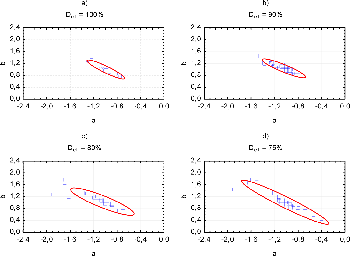
D-optimality: minimises the volume of the ellipsoidal confidence region of parameter estimates.

Plant friendliness requirements can be imposed in the form of input rate constraints, input and output magnitudes and experiment duration. We focus on input rate requirements, i.e., the input move range has to be smaller than a pre-specified tolerance. For discrete input signals, a quantitative plant friendliness index in terms of the number of changes from one level to another has been proposed [30]. For a deterministic sequence, the input plant friendliness component Φ_i can be defined as:

$${\Phi }_i=\left(1-\frac{n_t}{N-1}\right)$$

(1)

where N is the total length of an input signal and n_t is the total number of signal switchings. The above definition might be difficult to represent in the formulation of the optimisation problem. A closed form definition which retains the same intuitive appeal could be found in [21]:

$$\begin{array}{l}{\Phi }_i=1-\frac{{\displaystyle \sum {\left(u_k-u_{k-1}\right)}^2}}{\left(N-1\right)max{\left(u_k-u_{k-1}\right)}^2}\\ {\Phi }_i\approx 1,if{u}_k\approx u_{k-1},\forall k\le N\end{array}$$

(2)

where u_k, k = 1, …, N is an input sequence. For a continuous system, the definition of input friendliness can be modified as follows:

$${\Phi }_i=1-\frac{{\displaystyle \underset{0}{\overset{T}{\int }}{\dot{\mathbf{u}}}^T\dot{\mathbf{u}}}\text{d}t}{T\max \left({\dot{\mathbf{u}}}^T\dot{\mathbf{u}}\right)}$$

(3)

In many industrial applications a plant-friendly multi-sine input signal would be preferred for system identification. A multi-sine input is a signal obtained by the addition of a finite number of harmonically related sinusoids and can be represented as:

$$x\left(t\right)={\displaystyle \sum _{i=1}^{N_i}{a}_i\cos \left(2\pi k_{i}t/T+{\alpha }_i\right)}$$

(4)

where k_i are monotonically increasing harmonic numbers k_i ϵ N, i = 1, 2,…, N_i. The input friendliness factor is often expressed in terms of the peak factor Pf or the crest factor Cf:

$$Pf=\frac{x_{max}-x_{min}}{2\sqrt{2}{x}_{rms}}$$

(5)

$$Cf=\frac{max\left|x\right|}{x_{rms}}$$

(6)

where x_min, x_max, x_rms denote the minimum, maximum and rms values of the signal respectively. For a specified amplitude spectrum {a_i}, it is possible to synthesise an input signal with a low crest factor by using generalisation of the Polya’s algorithm [31].

3. Single Weighted Cost Function Method for a Time Domain Input Signal

We consider the problem of synthesising an optimal input in the time domain for plant-friendly identification. The system is described by the following state space model:

$$\begin{array}{l}\dot{\mathbf{x}}(t)=\mathbf{Ax}(t)+\mathbf{Bu}(t)\\ \mathbf{y}(t)=\mathbf{Cx}(t)+\mathbf{v}(t)\end{array}$$

(7)

where x is a n × 1 state vector, u is a m × 1 input vector, y is a r × 1 output vector, v is a r × 1 measurement noise vector, A (n × n), B (n × m), C (r × n) are, respectively: state, input and output matrices of the system. The vector v is a zero-mean Gaussian white noise process:

$$\begin{array}{l}E[\mathbf{v}(t)]=0\\ E[\mathbf{v}(t){\mathbf{v}}^{\mathrm{T}}(\tau )]=\mathbf{R}\delta (t-\tau )\end{array}$$

(8)

where R (r × r) is the covariance matrix of the measurement noise.

Let θ denote a k × 1 vector of unknown parameters to be estimated which is related with state space matrices A, B and C of the system. The Fisher information matrix (FIM) is defined as:

$$\mathbf{M}={\displaystyle \underset{0}{\overset{T}{\int }}{\mathbf{X}}_{\theta }^{\mathrm{T}}{\mathbf{C}}^{\mathrm{T}}{\mathbf{R}}^{-1}{\mathbf{CX}}_{\theta }}\mathit{dt}$$

(9)

where X_θ is an n × k parameter influence coefficient matrix with the ij-th component ∂x_i/∂θ_j.

For input design purposes, it is convenient to assume an unbiased estimator of θ, so that the covariance of the parameter estimates is given by the Cramer-Rao lower bound, viz., the inverse of the FIM. Then the covariance of the estimate ${\displaystyle \widehat{\mathbf{\theta }}}$ is:

$$\mathrm{cov}\left(\widehat{\mathbf{\theta }}\right)=E\left[\left(\widehat{\mathbf{\theta }}-\mathbf{\theta }\right){\left(\widehat{\mathbf{\theta }}-\mathbf{\theta }\right)}^{\mathrm{T}}\right]\ge {\mathbf{M}}^{-1}$$

(10)

The plant-friendly input signal is to be determined in such a way that the trace of the k × k Fisher information matrix (A-optimality) is maximized:

$$\mathrm{tr}(\mathbf{M})={\displaystyle \underset{0}{\overset{T}{\int }}\mathrm{tr}}\left[{\mathbf{X}}_{\theta }^{\mathrm{T}}{\mathbf{C}}^{\mathrm{T}}{\mathbf{R}}^{-1}{\mathbf{CX}}_{\theta }\right]\mathit{dt}$$

(11)

In order to maximise tr(M), let us define the augmented [(k + 1)n × 1] state vector [4]:

$${\mathbf{x}}_a={\left[\begin{array}{cccc}{\mathbf{x}}^{\mathrm{T}},& {\mathbf{x}}^{\mathrm{T}}{}_{\theta 1},& \cdots ,& {\mathbf{x}}^{\mathrm{T}}{}_{\theta k}\end{array}\right]}^{\mathrm{T}}$$

(12)

where x_θi = ∂x/∂θ_i. Then the state equation can be written as:

$${\dot{\mathbf{x}}}_a={\mathbf{A}}_a{\mathbf{x}}_a+{\mathbf{B}}_a\mathbf{u}$$

(13)

where the (k + 1)n × (k + 1)n matrix A_a and the (k + 1)n × m matrix B_a are given by:

(14)

$${\mathbf{B}}_a={\left[\begin{array}{cccc}\mathbf{B},& {\mathbf{B}}_{\theta 1},& \cdots ,& {\mathbf{B}}_{\theta k}\end{array}\right]}^{\mathrm{T}}$$

(15)

where A_θ = ∂A/∂θ_i and B_θ = ∂B/∂θ_i. In addition, we define C_a (rk × (k + 1)n) and R_a⁻¹ (rk × rk) as follows:

$${\mathbf{C}}_a=\left[\begin{array}{cccc}0& \mathbf{C}& 0& 0\\ ⋮& & \ddots & ⋮\\ 0& 0& 0& \mathbf{C}\end{array}\right]$$

(16)

$${\mathbf{R}}_a^{-1}=\mathrm{diag}\left({\mathbf{R}}^{-1}\right)$$

(17)

Then the expression for tr(M), given by Equation (11), can be written in the form:

$$\mathrm{tr}\left(\mathbf{M}\right)={\displaystyle \underset{0}{\overset{T}{\int }}{\mathbf{x}}_a^{\mathrm{T}}{\mathbf{C}}_a^{\mathrm{T}}{\mathbf{R}}_a^{-1}{\mathbf{C}}_a{\mathbf{x}}_a}\mathit{dt}$$

(18)

The objectives of the optimisation task should be as follows:

–

maximise tr(M),

–

maximise Φ_I as defined in Equation (3).

The cost function, which contains the input friendliness factor, can be expressed as:

$$J=\underset{\mathbf{u}}{\max }\frac{1}{2}{\displaystyle \underset{0}{\overset{T}{\int }}\left[{\mathbf{x}}_a^{\mathrm{T}}{\mathbf{C}}_a^{\mathrm{T}}{\mathbf{R}}_a^{-1}{\mathbf{C}}_a{\mathbf{x}}_a+\mu {\Phi }_i\right]}\mathit{dt}$$

(19)

where μ is the input friendliness factor constant. It must be noted that the time is not explicitly incorporated in the above cost function. Instead, the optimisation problem should be solved for different values of termination time. Let us introduce the input energy constraint:

$${\displaystyle \underset{0}{\overset{T}{\int }}{\mathbf{u}}^{\mathrm{T}}\mathbf{u}\mathit{dt}}\le E$$

(20)

Then, the cost function has the following representation:

$$J=\underset{\mathbf{u}}{max}\frac{1}{2}[{\displaystyle \underset{0}{\overset{T}{\int }}{\mathbf{x}}_a^{\mathrm{T}}{\mathbf{C}}_a^{\mathrm{T}}{\mathbf{R}}_a^{-1}{\mathbf{C}}_a{\mathbf{x}}_a\mathit{dt}}+\mu {\Phi }_i-q{\displaystyle \underset{0}{\overset{T}{\int }}\left({\mathbf{u}}^{\mathrm{T}}\mathbf{u}-\frac{E}{T}\right)}\mathit{dt}]$$

(21)

The case where μ = 0 has been solved in literature [4]. The multi-objective optimisation problem, corresponding to μ ≠ 0, can be solved by the Euler-Lagrange method which results in the following two-point boundary-value problem:

$$\frac{d}{\mathit{dt}}\left[\begin{array}{c}{\mathbf{x}}_a\\ \mathbf{\lambda }\\ \mathbf{u}\\ \dot{\mathbf{u}}\end{array}\right]=\left[\begin{array}{cccc}{\mathbf{A}}_a& 0& {\mathbf{B}}_a& 0\\ {\mathbf{C}}_a^{\mathrm{T}}{\mathbf{R}}_a^{-1}{\mathbf{C}}_a& -{\mathbf{A}}_a^{\mathrm{T}}& 0& 0\\ 0& 0& 0& \mathbf{I}\\ 0& \frac{{\mathbf{B}}_a^{\mathrm{T}}}{{\mu }^{\prime }}& \frac{q\mathbf{I}}{{\mu }^{\prime }}& 0\end{array}\right]\left[\begin{array}{c}{\mathbf{x}}_a\\ \mathbf{\lambda }\\ \mathbf{u}\\ \dot{\mathbf{u}}\end{array}\right]$$

(22)

where ${\mu }^{\dot{}}=\mu /\left(Tmax\left({{\displaystyle \dot{u}}}^{\mathrm{T}}{\displaystyle \dot{u}}\right)\right)$, and the boundary conditions are: x_a(0) = x_a0, λ(T) = 0, u(0) = u₀, ${\displaystyle \dot{u}}(T)=0$. The above differential equations are integrated to give u(t), using the method of complementary functions. However, calculation of the plant-friendly input signal requires the knowledge of the system parameters A, B, C and noise characteristics R. A common technique is to design the optimal inputs based on an initial estimate of the model parameters and improving the choice of the parameter values by iterative identification and experiment design [14].

The purpose of the current work is to formulate the optimisation problem for plant-friendly input design with respect to the D-efficiency constraint. In that way (i.e., by setting such a constraint to control the level of the D-optimality loss) we can obtain the friendliest input signal, reducing the rapid changes of the mass or energy inflow to the system.

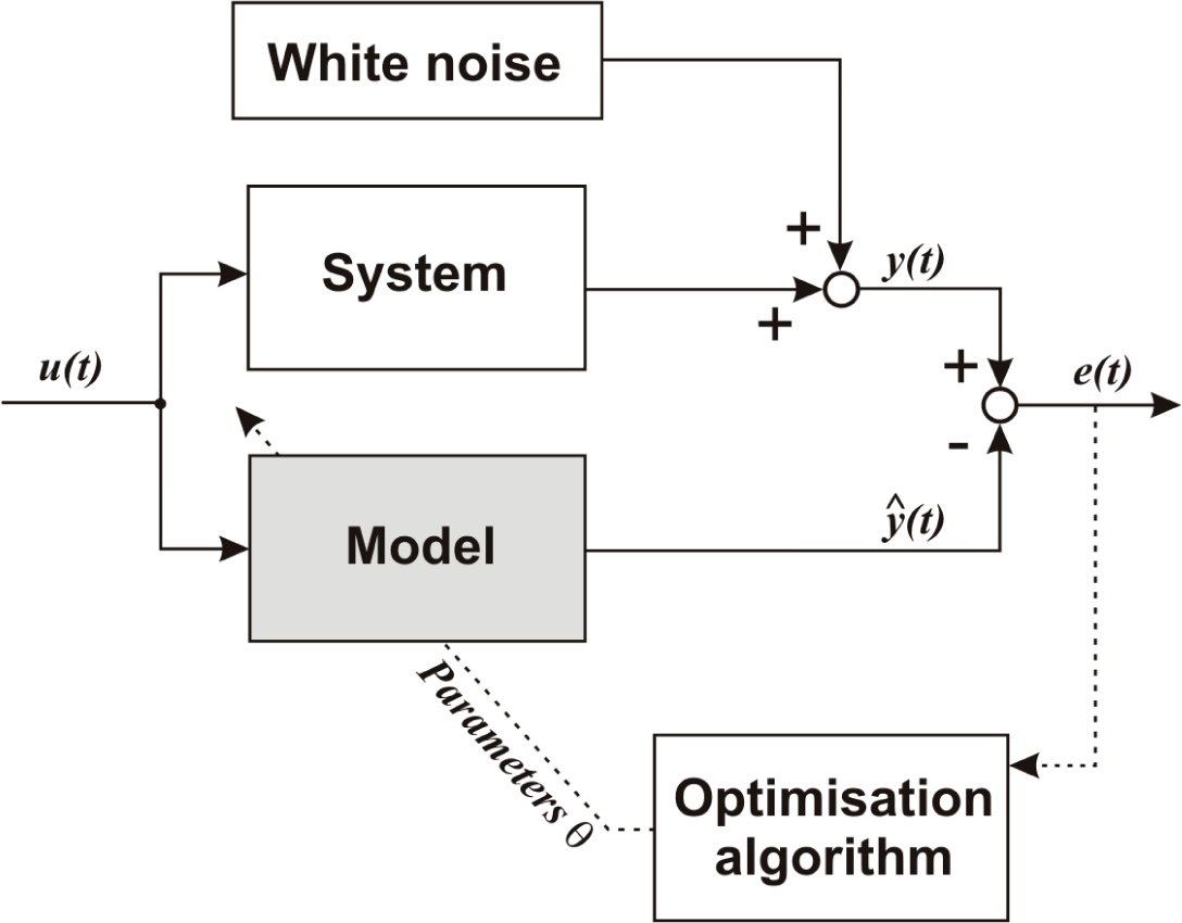
4. Plant Friendly Identification Problem Formulation

4.1. Input Friendliness Factor Formulation

For a continuous system, the definition of the input friendliness index Equation (3) can be modified as follows:

$${\Phi }_i=1-\frac{{\displaystyle \underset{0}{\overset{T}{\int }}({\dot{\mathbf{u}}}^{\mathrm{T}}(t)\dot{\mathbf{u}}(t))\mathit{dt}}}{\underset{0\le t\le T}{max}({\dot{\mathbf{u}}}^{\mathrm{T}}(t)\dot{\mathbf{u}}(t))}$$

(23)

The above plant friendliness factor maximisation is equivalent to minimisation of the following expression:

$$\frac{{\displaystyle \underset{0}{\overset{T}{\int }}({\dot{\mathbf{u}}}^{\mathrm{T}}(t)\dot{\mathbf{u}}(t))\mathit{dt}}}{\underset{0\le t\le T}{max}({\dot{\mathbf{u}}}^{\mathrm{T}}(t)\dot{\mathbf{u}}(t))}$$

(24)

For single-input and single-output (SISO) systems, let us introduce:

$$v(t):=\dot{u}(t)$$

(25)

and:

$$x_{n+1}(t):=u(t)$$

(26)

The above substitution can be interpreted as introducing the new state equation in the form:

$${\dot{x}}_{n+1}(t)=v(t),x_{n+1}(0)={\xi }_1$$

(27)

where ζ₁ is a parameter to be optimised.

Then the plant friendliness index (24) can be modified as follows:

$$\frac{{\displaystyle \underset{0}{\overset{T}{\int }}(v^{\mathrm{T}}(t)v(t))\mathit{dt}}}{\underset{0\le t\le T}{max}(v^{\mathrm{T}}(t)v(t))}$$

(28)

The above problem can be suitably modified by defining the plant friendliness index as:

$$\frac{1}{c}{\displaystyle \underset{0}{\overset{T}{\int }}\left(v^{\mathrm{T}}\left(t\right)v\left(t\right)\right)}\mathit{dt}$$

(29)

subject to:

$$\underset{0\le t\le T}{max}\left(v^{\mathrm{T}}\left(t\right)v\left(t\right)\right)\le c$$

(30)

Introducing another state variable x_n+2(t) = 1/c where ζ₂:= 1/c, we have:

$${\dot{x}}_{n+2}\left(t\right)=0,x_{n+2}\left(0\right)={\xi }_2$$

(31)

Then the problem (29) is equivalent to the canonical optimal control problem which maximises the performance index:

$${\displaystyle \underset{0}{\overset{T}{\int }}{x}_{n+2}(t)(v^{\mathrm{T}}(t)v(t))\mathit{dt}}$$

(32)

along with the inequality constraint:

$$x_{n+2}(t)(v^{\mathrm{T}}(t)v(t))\le 1,t\in [0,T]$$

(33)

The most suitable form to represent our problem is the Bolza functional form of the performance index, i.e., the sum of the terminal values of state variables and the integral of the control period. Such a typical form of the optimisation task allows obtaining the trajectory of the plant-friendly input signal with the use of one of existing software packages for solving numerically optimal control problems.

4.2. The D-Efficiency Constraint Formulation

The input signal employed in the identification experiment should simultaneously yield two results: acceptable accuracy of parameter estimates and making as spherical as possible the ellipsoidal confidence region of the estimates. Such a compromise can be reached applying an approach, which relies on the notion of the D-efficiency [29]. Any optimality criterion can be associated with the efficiency function, defined as a measure of the relative performance of any given experiment e compared to that of the optimal experiment e^*. The D-efficiency, which may be considered as a measure of the D-suboptimality of given input (plant-friendly) trajectories, is specified by:

$$E_D\left(\mathbf{e}\right)={\left\{\frac{\det \left(\mathbf{M}\left(\mathbf{e}\right)\right)}{\det \left(\mathbf{M}\left({\mathbf{e}}^{*}\right)\right)}\right\}}^{\raisebox{1ex}{$1$}\!\left/ \!\raisebox{-1ex}{$k$}\right.}$$

(34)

where k is the number of parameters to be identified, and e^* stands for the D-optimal trajectories which can be determined earlier. Following the reasoning and derivations presented in [32], we set a reasonable positive threshold η < 1 and impose the constraint on the D-efficiency value:

$$E_D\left(\mathbf{e}\right)\ge \eta$$

(35)

Such an approach will yield a D-suboptimal, yet reasonable solution. The inequality (35) is equivalent to the constraint:

$$\Psi \left[\mathbf{M}\left(\mathbf{e}\right)\right]\le D$$

(36)

where $\mathrm{\Psi }\left[{\displaystyle \mathbf{M}}\left({\displaystyle \mathbf{e}}\right)\right]=\log \left(\det {\displaystyle \mathbf{M}}\left({\displaystyle \mathbf{e}}\right)\right)$ and $D=\mathrm{\Psi }\left[{\displaystyle \mathbf{M}}\left({{\displaystyle \mathbf{e}}}^{*}\right)\right]-k{log}\left(\eta \right)$. The objective of such an experiment is formulated through maximisation of the FIM determinant (D-optimality) with respect to D-efficiency inequality constraint (36).

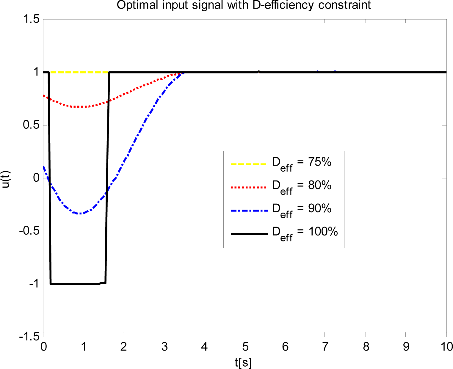
5. Plant-Friendly Identification with Respect to the Cost Function D-Efficiency Constraint

To illustrate the properties of the above approach to parameter identification, using the plant- friendly input signal and with respect to the assumed level of D-optimality, we have selected a simple first-order (inertial) object. The transfer function of an inertial model has the following form:

$$G\left(s\right)=\frac{k_p}{Ts+1}$$

(37)

The problem of synthesising a plant-friendly input signal with respect to the D-efficiency constraint for an inertial system can be described by the following single input, single output state space model:

$$\begin{array}{l}\dot{x}\left(t\right)=\mathit{ax}\left(t\right)+\mathit{bu}\left(t\right),x\left(0\right)=x_0\\ y\left(t\right)=x\left(t\right)\end{array}$$

(38)

where x = x(t, a, b) and model parameters a and b are constant. The principle of the design of optimal input signals for system identification is to maximise the sensitivity of the state variable or the observation to the unknown parameter [4]. The justification for this approach is the Cramer-Rao lower bound, which provides a lower bound for the estimation error covariance. Providing this feature of the input, we obtain the parameter estimate or observation sensitivity which tends to be lowered for an optimal input:

$$\mathrm{cov}\left(\left[a,b\right]\right)\ge {\mathbf{M}}^{-1}$$

(39)

The Fisher information matrix for the inertial model (38) can be expressed as:

$$\mathbf{M}\left(T\right)={\displaystyle \underset{0}{\overset{T}{\int }}\left[\begin{array}{c}{x}_a\\ x_b\end{array}\right]}\left[\begin{array}{cc}{x}_a& x_b\end{array}\right]\mathit{dt}={\displaystyle \underset{0}{\overset{T}{\int }}\left[\begin{array}{cc}{x}_a^2& x_a{x}_b\\ x_a{x}_b& x_b^2\end{array}\right]\mathit{dt}}=\left[\begin{array}{cc}{\displaystyle \underset{0}{\overset{T}{\int }}{x}_a^2\mathit{dt}}& {\displaystyle \underset{0}{\overset{T}{\int }}{x}_a{x}_b\mathit{dt}}\\ {\displaystyle \underset{0}{\overset{T}{\int }}{x}_a{x}_b\mathit{dt}}& {\displaystyle \underset{0}{\overset{T}{\int }}{x}_b^2\mathit{dt}}\end{array}\right]$$

(40)

where x_a = ∂x/∂a and x_b = ∂x/∂b. The problem can be suitably modified by defining the augmented state vector as [4]:

$${\dot{x}}_a=x+{\mathit{ax}}_a,x_a\left(0\right)=0$$

(41)

$${\dot{x}}_b={\mathit{ax}}_b+u,x_b\left(0\right)=0$$

(42)

A plant-friendly input signal for the inertial system perturbation is formulated through maximisation of the Fisher information matrix determinant (D-optimality) and the plant friendliness index maximisation in the form of a conventional integral-criterion optimal control problem. The problem of synthesising an optimal input signal for an inertial system, utilising Mayer’s canonical formulation of the performance index, has been solved in literature [26,27]:

$$\mathbf{M}(t)={\displaystyle \underset{0}{\overset{t}{\int }}\left[\begin{array}{c}{x}_a\\ x_b\end{array}\right]\left[\begin{array}{cc}{x}_a& x_b\end{array}\right]}\mathit{d\tau }//\frac{d}{\mathit{dt}}$$

(43)

the FIM can be modified as follows:

$$\dot{\mathbf{M}}(t)=\left[\begin{array}{c}{x}_a\\ x_b\end{array}\right]\left[\begin{array}{cc}{x}_a& x_b\end{array}\right],\mathbf{M}\left(0\right)=0$$

(44)

where:

$$\mathbf{M}\left(t\right)=\left[\begin{array}{cc}{m}_{11}\left(t\right)& m_{12}\left(t\right)\\ m_{21}\left(t\right)& m_{22}\left(t\right)\end{array}\right]$$

(45)

and:

$${\dot{m}}_{11}\left(t\right)=x_a^2\left(t\right),m_{11}\left(0\right)=0$$

(46)

$${\dot{m}}_{12}\left(t\right)={\dot{m}}_{21}\left(t\right)=x_a\left(t\right)x_b\left(t\right),m_{12}\left(0\right)=0$$

(47)

$${\dot{m}}_{22}\left(t\right)=x_b^2\left(t\right),m_{22}\left(0\right)=0$$

(48)

The augmented state Equations (41), (42), (46–48), taking into account input friendliness factor formulation (27), (31), are given by:

$$\begin{array}{lll}{x}_1=x,\hfill & {\dot{x}}_1={\mathit{ax}}_1+{\mathit{bx}}_7,\hfill & x_1\left(0\right)=x_{10}\hfill \\ x_2=x_a,\hfill & {\dot{x}}_2=x_1+a{x}_2,\hfill & x_2\left(0\right)=0\hfill \\ x_3=x_b,\hfill & {\dot{x}}_3=a{x}_3+x_7,\hfill & x_3\left(0\right)=0\hfill \\ x_4=m_{11},\hfill & {\dot{x}}_4=x_2^2,\hfill & x_4\left(0\right)=0\hfill \\ x_5=m_{12}=m_{21},\hfill & {\dot{x}}_5=x_2{x}_3,\hfill & x_5\left(0\right)=0\hfill \\ x_6=m_{22},\hfill & {\dot{x}}_6=x_3^2,\hfill & x_6\left(0\right)=0\hfill \\ x_7=u,\hfill & {\dot{x}}_7=v,\hfill & x_7\left(0\right)={\xi }_1\hfill \\ x_8=\frac{1}{c},\hfill & {\dot{x}}_8=0,\hfill & x_8\left(0\right)={\xi }_2\hfill \end{array}$$

(49)

Then the equivalent optimal control problem utilising Mayer’s canonical formulation, which maximises the performance index with respect to the D-efficiency equality constraint, is:

$$J=\left(x_4\left(T\right)x_6\left(T\right)-x_5^2\left(T\right)\right)-\mu {\displaystyle \underset{0}{\overset{T}{\int }}{x}_8(t)(v^T(t)v(t))\mathit{dt}}$$

(50)

subject to:

$$\begin{array}{l}{x}_8(t)(v^{\mathrm{T}}(t)v(t))\le 1,t\in \left[0,T\right]\\ \left(x_4\left(t\right)x_6\left(t\right)-x_5^2\left(t\right)\right)=D\\ -1\le x_7\left(t\right)\le 1\\ -{10}^4\le v\left(t\right)\le {10}^4\end{array}$$

(51)

where μ is the input friendliness factor constant and D is D-efficiency constant.

Note that in the above formulation v(t) (which is a derivate of the original control signal u(t)) acts as the input signal to the augmented system. We assumed the relatively wide range of the variability of v(t) to enable abrupt changes of the original control signal u(t), which is limited to the range of [−1, +1].

6. Experimental Results for the Inertial Case Study

For numerical solution of the above optimal control problems one of existing packages for solving dynamic optimisation tasks, such as RIOTS_95 [33], DIRCOL [34] or MISER [35], can be employed. We were employing the RIOTS_95 package, which is implemented in MATLAB, has efficient tools for solving the constrained problems of dynamic optimisation and can be easily merged with other MATLAB facilities (e.g., simulation of models developed in Simulink environment, with graphical user interface). All computations were performed using low-cost PC (Atom, 1.66 GHz, 1 GB RAM) running Windows 7 and MATLAB 7.12 (R2011a).

Optimal and sub-optimal signals were computed for nominal values of parameters: a = −1, b = 1 and with the termination time set as T_f = 10 s, using SQP algorithm. The system was assumed to be at the initial state x₁(0) = 5, the initial value of the control signal was chosen as u(0) = 1. The equations describing the system dynamics were integrated using the fixed step-size fourth-order Runge-Kutta method with grid intervals of 0.2 s. The D-optimal input signals obtained for different desired values of the D-efficiency constant D (according to Equation (36)) are shown in Figure 1. As the minimisation algorithms implemented in RIOTS_95 guarantee convergence only to a local minimum, we made use of the typical way to reduce the risk of “trapping”, i.e., repeating the computations several times, starting from different initial conditions from the range [−2.5, 2.5] around the “nominal” initial state x₁(0) = 5. The D-optimal excitation signal obtained when there was no constraint on the D-efficiency value (i.e., the coefficient η = 1 in the inequality (35)), is shown in black colour in Figure 1. It corresponds to the optimal experiment e^*, where the maximal possible value of the FIM determinant is obtained and in such a case the value D_eff = 100%·D_{eff, opt}. The control signals obtained for decreasing values of D-efficiency from the interval [75%, 100%] of its maximum value are shown in Figure 1. As we can see, when the desired value of D-optimality decreases, the shape of the optimal input signal substantially changes. While for the optimal experiment (in the sense of Equation (35)) there are the abrupt changes of the input, the control signal obtained for D_eff = 75%·D_{eff, opt} is almost constant, so the plant friendliness index increases to the value close to 1. The corresponding values of FIM determinant and plant friendliness index are displayed in

Table 1. Comparison of the performance index components.

Deff/Deff, opt	μ	D	J	Φi
100%	0.00	—	43.88	—
90%	50.00	35.60	32.03	0.88
80%	50.00	28.10	26.18	0.97
75%	50.00	25.00	25.00	1.00

.

The signals u(t) computed for different values of D-efficiency as solutions of the optimisation task (50) with the set of constraints (51), were then used as inputs in the parameter identification procedure. Figure 2 summarises the flow of information in the system identification process: we act on the physical system through the input u(t) and collect information through the observations of its output y(t). The presence of the white noise with different variance from the interval 0.0 ≤ σ² ≤ 0.8 makes the observations random variables. The model corresponds to the theoretical representation of the system (38), which depends on a vector of unknown parameters θ = [a, b]^T. The objective of the system identification task is to find the best values of model parameters θ in terms of the performance criterion. The ninety nine runs have been made for minimisation of the integral (within the time period from t₀ = 0 to the termination time T_f = 10 s) of the squared difference between the output of the system and the output of the model. The initial state of the inertial model was chosen from the interval –5 ≤ x₁(0) ≤ 5. The optimisation was performed using the Nelder-Mead method.

Figures 3a–d show the result of the simulation experiments, i.e., the optimal values of parameters computed as results of optimisation for each run, when the system starts from different initial state condition and the measurement noise influencing the system output has different variance.

Figure 3a shows the results with the input signal obtained for the maximal value of FIM determinant (i.e., D_eff = 100%·D_{eff, opt}), the successive figures show the results (for the same combinations of initial states and noise variance) with the input signals were computed when a certain loss of D-optimality was assumed as (D_eff/D_{eff, opt} = 90%, 80% and 75%, respectively).

Analysis of the confidence regions of the inertial model parameter estimates confirms the following regularities. The optimal input signal, obtained for D_eff/D_{eff, opt} = 100%, yields the minimal volume of the ellipsoidal confidence region of parameter estimates. When the desired ratio of D_eff/D_{eff, opt} decreases (i.e., we accept bigger loss of D-optimality), the cluster occupied by the optimal values of identified model parameters increases its size—for the same initial conditions and noise characteristics as in the above experiment. Decreasing the desired ratio of D_eff/D_{eff, opt} yields the input signal, which is more “friendly” for the plant, i.e., in that way we avoid abrupt changes of the control valve settings (or, changes of mass and energy flows) in the real-life identification experiments. The purpose of this case study was to show that the requirements of high friendliness of the input signal and the accuracy of parameter estimation are, in some sense, opposite.

7. Conclusions

A plant-friendly input signal design problem for system identification was formulated in the paper and the method of the problem solution was outlined. In the presented approach the input signal is a solution of a dynamic optimisation problem, where the plant friendliness index is maximised, at the same time providing a guaranteed level of D-efficiency. The goal of the study was to find the dependencies between the friendliness of the input signal used for identification of system parameters and the accuracy of parameter estimation, closely related to a desired level of D-efficiency. The identification experiments were performed in the presence of white noise of different variance (from a relatively wide range of values), which influenced the system output. The results obtained in the experiments give a qualitative picture of robustness of parameter estimation to the disturbances (which occur in practice, e.g., due to inaccurate measurements of the output signal) when the system is excited by a signal of a certain friendliness index.

The simple first-order inertial system case study of plant-friendly input signal design with guaranteed D-efficiency was presented in the paper. The D-optimal input signals were obtained for different values of the D-efficiency constant D and the maximum value of the input friendliness factor μ. The experiments confirm that we can provide a compromise between the friendliness of the plant excitation in the identification process and the accuracy of estimates (observed as a reasonably small volume of the confidence ellipsoid) for a wide range of measurement noise at the system output. One of the most important steps in the approach presented in the paper was the transcription of the proposed problem formulation into an equivalent optimal control task expressed in the Lagrange form with the appropriate set of constraints. The optimal input trajectories were then computed using one of existing packages for solving dynamic optimisation problems. A plant-friendly input signal design for solving free final time parameter estimation problem will be presented.

References

1. Godfrey, K. Perturbation Signals for System Identification; Prentice-Hall: Englewood Cliffs, NJ, USA, 1993. [Google Scholar]
2. Ljung, L. System Identification: Theory for the User; Prentice-Hall: Englewood Cliffs, NJ, USA, 1999. [Google Scholar]
3. Pintelon, R.; Schoukens, J. System Identification: A Frequency Domain Approach; John Wiley & Sons: New York, NY, USA, 2001. [Google Scholar]
4. Kalaba, R.; Spingarn, K. Control, Identification, and Input Optimization; Plenum Press: New York, NY, USA, 1982. [Google Scholar]
5. Mehra, R. Choice of Input Signals. In Trends and Progress in Systems Identification; Eykhoff, P., Ed.; Pergamon Press: New York, NY, USA, 1981. [Google Scholar]
6. Hugo, A.J. Process controller performance monitoring and assessment. Control. Arts Inc. 2001. Available online: http://www.controlarts.com/ accessed on 20 March 2014.
7. Ren, M.; Wu, D.; Zhang, J.; Jiang, M. Minimum entropy-based cascade control for governing hydroelectric turbines. Entropy 2014, 16, 3136–3148. [Google Scholar]
8. Meng, Q.; Fang, F.; Liu, J. Minimum-information-entropy-based control performance assessment. Entropy 2013, 15, 943–959. [Google Scholar]
9. Walter, E.; Pronzato, L. Qualitative and quantitative experiment design for phenomenological models-a survey. Automatica 1990, 26, 195–213. [Google Scholar]
10. Pronzato, L.; Thierry, E. A minimum-entropy estimator for regression problems with unknown distribution of observation errors; Research Report 00–08, Laboratoire d’Informatique, Signaux et Syst’emes I3S-UMR6070-UNSA; CNRS: Sophia-Antipolis, France, 2000. Available online: http://www.i3s.unice.fr/%7Epronzato/biblio.html accessed on 20 March 2014.
11. Wolsztynski, E.; Thierry, E.; Pronzato, L. Minimum-entropy estimation in semi-parametric models. Signal Process 2005, 85, 937–949. [Google Scholar]
12. Indiveri, G. An entropy-like estimator for robust parameter identification. Entropy 2009, 11, 560–585. [Google Scholar]
13. Zarrop, M.B. Optimal Experiment Design for Dynamic System Identification; Lecture Notes in Control and Information Sciences; Volume 21, Springer-Verlag: Berlin, Germany, 1979. [Google Scholar]
14. Antoulas, A.; Anderson, B. On the choice of inputs in identification for robust control. Automatica 1999, 35, 1009–1031. [Google Scholar]
15. Gevers, M.; Ljung, L. Optimal experiments designs with respect to the intended model application. Automatica 1986, 22, 543–554. [Google Scholar]
16. Hildebrand, R.; Gevers, M. Identification for control: Optimal input design with respect to worst-case v-gap cost function. SIAM J. Control Optim. 2003, 41, 1586–1608. [Google Scholar]
17. Pronzato, L. Optimal experimental design and some related control problems. Automatica 2008, 44, 303–325. [Google Scholar] [Green Version]
18. Hussain, M. Review of the applications of neural networks in chemical process control-simulation and on-line implementation. Artif. Intell. Eng. 1999, 13, 55–68. [Google Scholar]
19. Narasimhan, S.; Rengaswamy, R. Multi-objective input signal design for plant friendly identification of process systems. Proceeding of the American Control Conference, Boston, MA, USA, 30 June–2 July 2004; pp. 4891–4896.
20. Narasimhan, S.; Rengaswamy, R. Multi-objective optimal input design for plant friendly identification. Proceeding of the American Control Conference Seattle, Washington, WA, USA, 11–13 June 2008; pp. 1304–1309.
21. Rivera, D.; Braun, M.; Mittelmann, H. Constrained multisine inputs for plant friendly identification of chemical process. Proceeding of the IFAC World Congress, Barcelona, Spain, 21–26 July 2002.
22. Rivera, D.; Lee, H.; Braun, M.; Mittelmann, H. Plant friendly system identification: A challenge for the process industries. Proceeding of the SYSID 2003, Rotterdam, The Netherlands, 27 August 2003.
23. Steenis, R.; Rivera, D. Plant-Friendly Signal Generation for System Identification Using a Modified Simultaneous Perturbation Stochastic Approximation (SPSA) Methodology. IEEE Trans. Control Syst. Technol. 2011, 19, 1604–1612. [Google Scholar]
24. Rivera, D.; Lee, H.; Mittelmann, H.; Braun, M. Using plant-friendly multisine signals to identify a strongly interactive process. IEEE Control Syst. Mag. 2007, 27, 72–89. [Google Scholar]
25. El-Kady, M.; Salim, M.; El-Sagheer, A. Numerical treatment of multiobjective optimal control problems. Automatica 2003, 39, 47–55. [Google Scholar]
26. Jakowluk, W. Design of an optimal excitation signal for identification of inertial systems in time domain. Przegląd Elektrotechniczny 2009, 85, 125–129. [Google Scholar]
27. Jakowluk, W. D-Optimal Experiment Design for Estimating Parameters of Dynamic Systems. Ph.D. Dissertation, Faculty of Electrical Engineering, Bialystok University of Technology, 2008. [Google Scholar]
28. Jakowluk, W. Design of an optimal actuation signal for identification of a torsional spring system. Przegląd Elektrotechniczny 2011, 87, 154–160. [Google Scholar]
29. Atkinson, A.; Donev, A.; Tobias, R. Optimum Experimental Design with SAS; Oxford University Press: Oxford, UK, 2007. [Google Scholar]
30. Parker, R.; Heemstra, D.; Doyle, F.; Pearson, R.; Ogunnaike, B. The identification of nonlinear models for process control using tailored “plant-friendly” input sequences. J. Process Control 2001, 11, 237–250. [Google Scholar]
31. Guillaume, P.; Schoukens, J.; Pintelon, R.; Kollar, I. Crest-factor minimization using nonlinear Chebyshev approximation methods. IEEE Trans. Instrum. Measur. 1991, 40, 982–989. [Google Scholar]
32. Uciński, D.; Chen, Y.Q. Sensor Motion Planning in Distributed Parameter Systems Using Turing’s Measure of Conditioning. Proceedings of the 45th IEEE Conference on Decision and Control, San Diego, CA, USA, 13–15 December 2006; pp. 759–764, WeB03.6, (published on CD-ROM).
33. Schwartz, A.; Polak, E.; Chen, Y. A. MATLAB toolbox for solving optimal control problems. Version 1.0 for Windows. May 1997. accessed on 20 March 2014. Available online: http://www.schwartz-home.com/RIOTS/.
34. Stryk, O. User’s quide for DIRCOL, a direct collocation method for the numerical solution of optimal control problems. Version 2.1; Technische Universität Darmstadt: Germany, November 1999. accessed on 20 March 2014. Available online: http://www.sim.informatik.tu-darmstadt.de/index/leftnav.html.
35. Jennings, L.; Fisher, M.; Teo, K.; Goh, C. MISER 3: Optimal control software. Version 2.0; Theory and user manual. Dept. of Mathematics, University of Western Australia: Nedlands, 2002. Available online: school.maths.uwa.edu.au/~les/miser/Misermanual.pdf accessed on 20 March 2014.
Figure 1. Optimal and sub-optimal input signals to the inertial system for different D-efficiency values.
Entropy 16 05822f1
Figure 2. Flow of information in the parameter identification system.
Entropy 16 05822f2
Figure 3. Confidence regions of the inertial model parameter estimates; the model was excited utilising: (a) Optimal input signal (Deff = Deff, opt); (b) Sub-optimal input signal (Deff = 90%·Deff, opt); (c) Sub-optimal input signal (Deff = 80%·Deff, opt); (d) Sub-optimal input signal (Deff = 75%·Deff, opt).
Entropy 16 05822f3