Applying Information Theory to Neuronal Networks: From Theory to Experiments

 ,
,
Abstract
: Information-theory is being increasingly used to analyze complex, self-organizing processes on networks, predominantly in analytical and numerical studies. Perhaps one of the most paradigmatic complex systems is a network of neurons, in which cognition arises from the information storage, transfer, and processing among individual neurons. In this article we review experimental techniques suitable for validating information-theoretical predictions in simple neural networks, as well as generating new hypotheses. Specifically, we focus on techniques that may be used to measure both network (microcircuit) anatomy as well as neuronal activity simultaneously. This is needed to study the role of the network structure on the emergent collective dynamics, which is one of the reasons to study the characteristics of information processing. We discuss in detail two suitable techniques, namely calcium imaging and the application of multi-electrode arrays to simple neural networks in culture, and discuss their advantages and limitations in an accessible manner for non-experts. In particular, we show that each technique induces a qualitatively different type of error on the measured mutual information. The ultimate goal of this work is to bridge the gap between theorists and experimentalists in their shared goal of understanding the behavior of networks of neurons.1. Introduction
In the field of complexity and complex systems research there is a growing interest in the use of information theory (IT) as a principal tool in the development of new theories [1–11]. In this article we are concerned with the information theory based on probability densities, primarily that of Shannon [12,13]. Applications of information theory to complex systems research range from the pragmatic viewpoint, such as using the mutual information function as a non-linear correlation measure, to the more fundamental viewpoint intended here, where each dynamical system is interpreted as a (Turing) computation, consisting of the storage, transfer, and modification of information. In the latter work, informational bits are considered to be physically stored in the states of dynamical components (neurons) at one instant. The fundamental question is then: where does each bit go? Tracing how informational bits flow through a dynamical system (e.g., a network of neurons) is anticipated to reveal important characteristics about the system, such as which components (neurons) are the most influential [14]; whether two “colliding” pieces of information [15] become integrated or; or whether the dynamical behavior at large is stable (resilient to perturbation) or unstable [16,17], to name examples. The theory needed to fully trace the information through a dynamical system is still under development. The basic building blocks of such theoretical work are Shannon’s entropy and mutual information functions. Based on these measures a wide range of information-theoretical measures have been derived, such as information redundancy, multi-information, information synergy [9,10,18], and (localized) Transfer Entropy [19,20]. The list of derived measures grows steadily as the necessary “information processing” theory is being developed.
Theory should lead to hypotheses which can be tested experimentally, and vice versa, experiments should inspire new theoretical development. It is therefore crucial that bridges are built between theorists and experimentalists, translating theoretical measures to valid experimental setups, and simultaneously, understanding the effect of different experiments on the measurement of information-theoretical quantities. It is the belief of the authors that the current research into the elusive “information processing” theory is focused heavily on theoretical work and computer modeling, and could benefit from both hypothesis building from experimental results as well as experimental testing of ideas. Conversely, the authors believe that experimentalists tend to focus on a set of de facto canonical measurements of correlation, such as linear (VAR-based) Granger causality and Fourier-transform-based measures, and could indeed benefit from the development of new theories and measures of dependence and different types of interaction.
The purpose of this article is to help build such a bridge for the domain of networks of neurons, also known as neuronal microcircuits. Networks of neurons are a paradigmatic example where emergent, complex behavior arises from relatively simple elements. Although each individual neuron has complicated machinery with non-trivial dynamics of its own, the systemic behavior of a (large) network of such neurons can in no way be predicted by extrapolating the dynamics of a single neuron. The structure of the network of interactions among the neurons thus plays an important role in generating complex behavior, but exactly how the individual dynamics and network structure complement each other is poorly understood. The purpose of this article is to pave the way for the experimental validation of theories based on information theory, which are intended to address these problems.
Concretely this article consists of two parts. In the first part we will describe two suitable experimental techniques for the measurement of information-theoretical quantities in local networks of individual neurons. We also argue why other techniques are less suited for this task. One important conclusion from this part is that the two suitable experimental techniques each comes with a different drawback in terms of measurement accuracy. Therefore, in the second part of this article we study numerically the error induced by both techniques. In particular, we are interested in the question whether the two types of induced measurement error are qualitatively different in nature or not, i.e., we are not interested in a faithful, quantitative characterization of the induced error. As a first answer to this question we focus on a single pair of neurons, which we model by a prior and conditional probability distribution which are induced by the local network that surrounds them. Then we calculate numerically the pairwise mutual information both exactly (error-free null hypothesis) as well as after modeling the measurement error induced by each technique. Most derived measures, such as Transfer Entropy, can be expressed in terms of pairwise mutual information quantities, which is the reason we focus on the pairwise case. Finally we will discuss the qualitative differences between the two results, which demonstrate that the experimental technique must be selected carefully based on the goal of the study. Further study is needed to understand more accurately what error is induced in derived information-theoretical measures.
We emphasize explicitly that it is not our goal to find improved measures of (directed) causal dependence over, e.g., the well-known Granger causality or partial directed coherence, which are often used in search of the so-called “effective connectivity” between neurons. Although certain derived information-theoretical measures are indeed proposed in this context, such as Transfer Entropy, our goal is more general, namely to stimulate the experimental measurement of any derived measure, and conversely, to propose new hypothesized measures in the more general search for a theory of “information processing” in complex dynamical systems.
2. Experimental Techniques
There are many techniques available to measure either the topology or the dynamics of a neuronal network independently. For a technique to be considered for use with IT, it must be able to simultaneously measure both: (i) the dynamics of each individual cell as a time series, and (ii) the location of the corresponding individual cell in the microcircuit. This is because the developing “information processing” theory is concerned with explaining the role of the neuronal network structure on the dynamics of the network in a bottom-up manner: namely, concerning how the network induces a flow of individual bits [8,11,14,16,17,21], as well as the interaction between bits into higher-level information [11,16,18].
Among the techniques that do not satisfy these requirements are fMRI and EEG. They are well-known, non-invasive techniques that have been used extensively in topology versus dynamics research in brain networks on a high cognitive level, i.e., measuring the activity of very large conglomerates of cells [22]. Both techniques suffer from a spatial resolution limitation that does not allow for determining either the location or the dynamics of individual cells. On the other hand, simultaneous intracellular recordings can be made from multiple different cells in a network [23]. The number of cells that can be measured simultaneously, however, is limited by, among others, the mechanical and biophysical instabilities of the cells as well as the recording instruments. Every neuron is impaled by a glass electrode that is mounted on an adjustable microcontroller. The microcontrollers are bulky and do not allow for more than four intracellular recordings simultaneously, due to lack of space. Furthermore cells in vitro still move slightly, which might cause the membrane to rip, leading to death of the cell. Because of these limitations we do not consider multiple simultaneous cell recordings as a viable technique to use with IT.
We will discuss in more detail two different techniques that are capable of satisfying the above-mentioned requirements to work with IT. These are calcium imaging and multi-electrode arrays, and are used on cultured neuronal networks and in behaving animals.
2.1. Calcium Imaging
Calcium imaging (CI) relies on calcium ions to rapidly increase the membrane potential to generate an action potential (AP). By introducing into neurons a fluorescent dye that binds to calcium, the concentration of Ca2+ inside the cell can be monitored by imaging the cell(s) with a laser that excites the dye, thereby inferring the cell’s activity reflected in changes in Ca2+. CI allows functional imaging in vitro (brain slices (24) as well as cultured networks) and in vivo on single cell level resolution [25,26], with near-millisecond precision [27] and a depth penetration of several hundreds of microns [28], making it possible to measure multiple layers of cells.
2.1.1. Methodology
CI can be used on single cells and circuits. Because we are interested in network behavior, we look at circuits rather than single cells. Gobel and Helmchen [28] describe four ways to administer the Ca2+ indicator in and/or around the cells. A typically used technique is called multi-cell bolus loading (MCBL). In MCBL a Ca2+ indicator is pressure-injected into a brain area. The commonly used Ca2+ indicators (e.g., Oregon Green 488 BAPTA-1 acetoxymethyl ester [OG-1 AM]) are modified to have acetoxymethyl (AM) esther-groups. These lipophilic groups allow the otherwise lipophobic dye molecules to pass the lipid-rich cell membrane allowing the indicator to be taken up into the cell, where it can be bound only by Ca2+ present in the intracellular compartment. Enzymes present inside the cells (cytosolic esterases) remove the AM-groups inside the cell, forcing the dye molecules to remain in the intracellular compartment. This process is called intracellular de-esterification of acetoxymethyl ester derivatives and it makes the cell membrane impermeable for the indicator, thereby trapping the indicator inside the cell. After administration the indicator accumulates within the cells, enhancing the fluorescence contrast between the cells and the extracellular compartment [29]. This technique can also be easily used in vitro, on cultured networks, by exposing the cells to the indicator under well-defined experimental conditions.
A different technique to introduce the indicators in the cell is by use of genetically encoded Ca2+ indicators (GECI), i.e., indicators that are being synthesized by the cell itself. By inserting a gene into the cells’ DNA, this transgene forces the cell to synthesize a protein with fluorescent properties, which is at the same time sensitive to fluctuations in intracellular Ca2+ concentrations. While this approach has some very attractive properties (such as cell-specificity) it is suffers from limitations such as relatively small dynamic ranges, slow response kinetics in vivo and non-linear behavior that makes interpretation of its fluorescence non trivial [30]. Moreover, as transfection efficacy is rarely 100%, the technique does not allow for observation of the whole network, unless stable cell lines are made, which is virtually incompatible with the common use of primary neurons for neuron network analysis. Stable cell lines are neurons that have been cloned and transfected multiple times until a set percentage of the cells have then inserted gene and express the protein, while primary neurons come directly from the tissue [31]. For more details and references to these (and other) methods see [28] for an overview on CI methods and [30–32] for an extensive overview on genetic methods.
2.1.2. Output
CI produces time series of fluorescence images in a defined area. Because CI tracks an indirect measure of activity, the output differs from the original signal in two ways: (i) a time lag in the onset of activity signals, and (ii) a smearing factor in the decay of the signal reference. While the Ca2+ influx may be directly linked with the triggering of an AP and is therefore aligned with the activity inside the cell, the emitted fluorescence builds up over time and therefore lags behind the original activity, thus it is a surrogate measure of the initial variable. The smear in the decay of the signal is caused by the gradual decrease in Ca2+ concentration. After the AP has been fired, the membrane potential drops very quickly (~10 ms) due to influx of K+ ions. The Ca2+ concentration does not decrease with the same speed (in the range of 200 ms), because it is limited by the speed at which Ca2+ ions are pumped out of the cell. Some cells fire many APs in a short time (e.g., bursting neurons) leading to a build-up of fluorescence, that make it difficult to determine the exact number of APs [33].
In the specific case of measuring the topology of a network, it could be enough to video-record the network activity over time. The active neurons are visible when they fire and by analyzing the resulting images, the topology of the network could be reconstructed, e.g., using IT tools [34]. In order to experimentally observe active axons and dendrites, and thus trace the topology of the network without an inference step, additional stainings are possible [35] in order to visualize the active synapses.
2.2. Multi Electrode Arrays
Multi electrode arrays (MEAs) contain multiple electrodes that measure voltage fluctuations in the extracellular environment. MEAs are non-cell-invasive and can be used in vitro [36] as well as in vivo (with so called polytrodes) to make multi-channel recordings with a very high temporal resolution [37]. In vitro MEAs can contain up to 10,000 electrodes and in vivo the polytrode is limited to about 100 electrodes. Under ideal situations, recording can last for weeks without damaging the cells membranes, allowing the study of the network activity in time. Current developments allow for in vitro recordings in 3D networks [38].
2.2.1. Methodology
MEAs record field potentials (FPs), sometimes also called local field potentials (LFPs). FPs are an attenuated and temporarily filtered reflection of the activity of cells surrounding the electrode. Reconstructing the sources of FPs is possible because the processes behind their generation are known. Separating spike trains is also possible from MEA data, as shown by Meister, Pine and Baylor who made parallel recordings from 61 sites on an MEA and, by means of an offline spike sorting algorithm, separated spike trains from up to 100 neurons [37].
2.2.2. Output
MEA output is a time series of voltages for every electrode. MEAs have a very good temporal resolution, but in order to extract spikes and attribute them to separate neurons MEA data needs extensive data processing. These techniques/algorithms continue to improve in terms of speed and reliability [39]. While spike sorting algorithms improve their precision, (i) it remains difficult to sort spikes further away from the electrode, resulting in multi-unit activity [40], (ii) low frequency firing neurons are not considered (due to high- and low-pass filtering) while they carry a high amount of information (because of their selectivity) and (iii) cluster stability (movement of the electrode over time for instance due to growth of the network) limits automatic spike sorting algorithms when using recordings over periods longer than weeks, introducing the need for manual work and therefore subjectivity [39].
The introduction of the MEA (as compared to earlier used tetrodes) has increased the number of neurons that we measure immensely, leading to difficulties efficiently and correctly identifying the location of a neuron based on the spiking pattern recorded by the MEA. When using MEA data with IT, the uncertainty about the exact location of the neuron must be taken into account.
Although MEA does not allow measuring the topology of active synapses directly, its spatial and temporal resolution of recording spike trains allow inferring the effective connectivity with relatively high precision [41].
2.3. Comparison of Techniques
In this section differences between the two techniques are discussed. A brief summary can be found in Table 1.
2.3.1. Temporal/Spatial Resolution and Challenges
As briefly discussed before, Ca2+ flux is an indirect measure of the actual electrical mechanisms in the neuron. Consequently, fluorescent Ca2+ indicators generally fail to register sub threshold activity—electrical inputs to the neuron that do not lead to an action potential. In addition, Ca2+ is a slow signal that lags behind electrical activity [32]. MEA has a very good temporal resolution in comparison, because electrical signals travel through the extra-cellular medium very quickly and can be measured almost instantly. The spatial resolution is MEAs weakness because the electrodes are surrounded by cells and do not connect to one specific neuron. Therefore, it is possible to receive the same input from two different neurons, provided that these neurons are at the same distance from the electrode. The location of a neuron is also not directly measured, so in order to extract the location of a neuron, MEAs rely on algorithms and therefore the topology is only as reliable as the algorithm.
2.3.2. Invasiveness
Both CI and MEA are considered cell non-invasive, i.e., neurons are not injured when measuring with these techniques. Animals do need to undergo surgical operations in order to make the experiments possible [25,42]. Regarding CI, after injecting the fluorescent dye the brain area can be monitored for a couple of hours in living animals as well as in neuronal cultures and brain slices [30]. MEAs are placed in the extracellular environment and therefore do not damage the cells. The brain area continues to function normally and recordings can last for days to months [43].
2.3.3. Number of Cells Measured
While theoretically the spatial range of CI is only limited by the size of the signal and the wavelength of the light used [44], good results have been reported of recording up to 150 neurons [45]. MEAs only measure a (small) proportion of neurons in an area, limited by the size of the array and the number of electrodes on the array. Technological developments have the potential to record from thousands of neurons simultaneously in vivo, but new spike sorting algorithms are needed to interpret this data. With current methods ~200 neurons can be recorded simultaneously in vivo [39].
2.3.4. Cell Specificity
The fluorescent dye can be taken up by not just neurons and therefore it is difficult to tell the difference between neurons and glia cells when using CI. At the same time it must be mentioned that the nature of Ca2+ dynamics are characteristic of neurons, since they originate from action potentials, which are not present in astrocytes. Genetical indicators are a promising technique to enhance differentiation of cells, by targeting the expression of the indicator specifically to neurons, or groups of them, using specific gene promoters. Because MEAs record in the extracellular environment, they cannot differentiate between different types of cells, however, the electrical characteristics of the recordings made could be used in some cases to identify specific cell populations. A certain brain area comprises of multiple types of neurons and MEAs will simply record the superposition of all their signals.
2.3.5. Blindness
Both CI and MEA are functionally blind for cells that are silent (do not fire). CI is capable of showing sub-threshold fluctuations but these are small signals and therefore susceptible to noise. MEAs only measure the activity of excitatory cells, because they are the only cells that spike and therefore the only kind whose activity is reflected in the extracellular medium.
3. Information Theory: Measuring from Experiments
From the previous section it is clear that MEA and CI each will have a different type of error in the measurement of neuronal activity. MEA measures spikes accurately in the temporal dimension but cannot measure directly which neuron generated the spike; CI measures accurately which neuron generates a spike, but may miss consecutive spikes due to the temporal “smearing” effect. We develop two simple models of the measurement error induced by the MEA and CI techniques and study numerically their impact on the measured pairwise mutual information between two neurons. We focus on pairwise mutual information because many derived information-theoretical measures can be written as a sum of (conditional) pairwise terms.
The purpose of the two models is to qualitatively compare the effect of the measurement on the mutual information, in order to determine whether one technique is merely a more accurate variant of the other, or whether the two types of techniques are qualitatively different and possibly complementary. In the latter case the choice of experiment crucially depends on the higher-level goal of the study, such as calculating information synergy or inferring the strengths and direction of the anatomical links. Each model by itself is explicitly not intended to be an accurate description of the measurement error of the corresponding technique, but it is expected to give us more qualitative insight into the error in each experimental technique.
3.1. Information Theory Metrics
In order to model a neuron’s activity we define it as a binary random variable X that takes the values X =1 if the neuron is firing or X=0 if the neuron is not firing in a given time interval. The Shannon entropy is a measure of the uncertainty of a random variable and is defined as:
Mutual information, I, is a common measure of the dependence between two variables. It quantifies the reduction of the uncertainty of variable X when we have knowledge of a variable Y.
The mutual information between two variables X and Y is defined as:
Two interconnected neurons should have a non-zero mutual information since one neuron partially determines the state of the other neuron. On the other hand, two independent variables would not share any mutual information and so that their mutual information is zero.
3.2. Mutual Information between Two Neurons
The mutual information of two neurons N1 and N2 with prior probabilities of firing in a given small time interval are P(N1=1)=p and respectively, and conditional probabilities P(N2=1|N1=1)=q1 and P(N2=1|N1=0)=q0 is:
The limitations of the two experimental measurement techniques, mentioned above, introduce different types of errors in the measurement of the mutual information. In the following section we will try to model and compare these two different types of errors.
Furthermore this result can be generalized using the chain rule of mutual information. The mutual information of a local network of neurons can be decomposed into a sum of (conditional) pairwise mutual information terms, where each of which will have a different qq but the total error can still be estimated using the methods in this section.
3.3. Error in Multi-Electrode Array
The existence of more than one neuron around each electrode in a MEA introduces uncertainty when trying to distinguish between them. When a spike is detected by an electrode it must be assigned to one of the nearby neurons. While algorithms designed for this task are getting more and more precise [39], the assignment is not yet perfect [40], leading to a certain probability for a false positive (an assigned spike to a neuron that did not fire) and a false negative (no assigned spike for a neuron that fired).
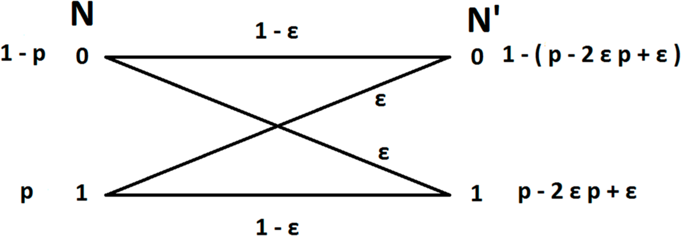
In order to model the error induced by the effect of spike miss-assignment we will consider the measurement as being a transmission over a binary symmetric channel (Figure 1). This means that a neuron fires with probability P(N = 1) and does not fire with probability P(N = 0).Then we consider the measurement N′ as the probability of assigning a spike to the neuron P(N′ = 1) and the probability of not assigning a spike to the neuron P(N′ = 0).
Now we consider the measurement error as the probability to miss-assign a spike to a neuron. Considering the high accuracy of modern techniques we assume that this probability is small. This means that when a neuron fires with probability P(N = 1) = p the probability of falsely assigning this spike to another neuron, and thus not assigning a spike to the firing neuron, is the conditional probability P(N′ = 0 | N = 1) = ε, and the probability of correctly assigning a spike to the firing neuron is P(N′ = 1 | N = 1) = 1‒ε. Similarly when a neuron does not fire P(N = 0) = 1 ‒ p the probability of a false positive, i.e., that a spike from a different neuron will be assigned to it is P(N′ = 1 | N = 0) = ε and the probability of correctly not assigning a spike to the neuron is P(N′ = 0 | N = 0) = 1 ‒ ε.
Then the probability of assigning a spike to a neuron that fires with probability P(N = 1) = p is: P(N′ = 1) = P(N′ = 1 | N = 1)P(N = 1) + P(N′ = 1 | N = 0)P(N = 0) = (1 ‒ ε)p + ε(1 ‒ p) = p ‒ 2εp + ε and the probability of not assigning a spike to that neuron is: P(N′ = 0) = P(N′ = 0 | N = 1)P(N = 1) + P(N′ = 0 | N = 0)P(N = 0) = εp + (1 ‒ ε)(1 ‒ p) = 1 ‒ (p ‒ 2εp + ε).
With this knowledge we can compute the measurement error in mutual information due to spike miss-assignments. The choice of the value for parameter εε is induced by the experimental setup and the neuronal network, such as the density of neurons around electrodes, the density of their spiking activity, and the offline algorithm for assigning spikes to neurons.
3.4. Error in Calcium Imaging
On the other hand measuring mutual information with CI leads to a different type of error. With this experimental method we can always correctly assign a spike to the neuron that fires. The error arises from the slow signal of the fluorescence of a neuron following a spike, which lasts roughly an order of magnitude longer than the duration of a single spike. Considering that neurons tend to spike in bursts there is a non-negligible probability that two or more spikes will be temporally close together in such a way that the second spike will not be detected by the fluorescence processing software. This will lead to a “shadowing effect”, such that one spike causes another spike to be missed.
In order to quantify this measurement error, we divide the measurement time into Ñ bins of equal duration—suitably chosen depending on the experimental details—and assume that in one such bin there can either be zero, one or two spikes. We further define α to be the probability that two spikes appear in one bin, given that at least one spike has been detected in the bin.
Under these assumptions there are four events that can be measured regarding each neuron of the pair for which we aim to calculate the mutual information: both neurons spike (P11), only the first spikes (P10), only the second spikes (P01), and neither spikes (P00). That is, the measurement cannot distinguish between single and double spikes for each neuron, so there are the four observable events out of the nine possible ones. We designate the probabilities for these events to occur as , , and respectively. We evaluate these probabilities by counting the number of occurrence of each of these events. The effect of not being able to detect the difference between a single and double spike is to reduce the effective count of events from the true ones. Taking this into account, one can then show that the relation between the true joint probabilities (without tilde) and the measured ones (with tilde) is:
3.5. Comparison of the Two Measurement Error Models
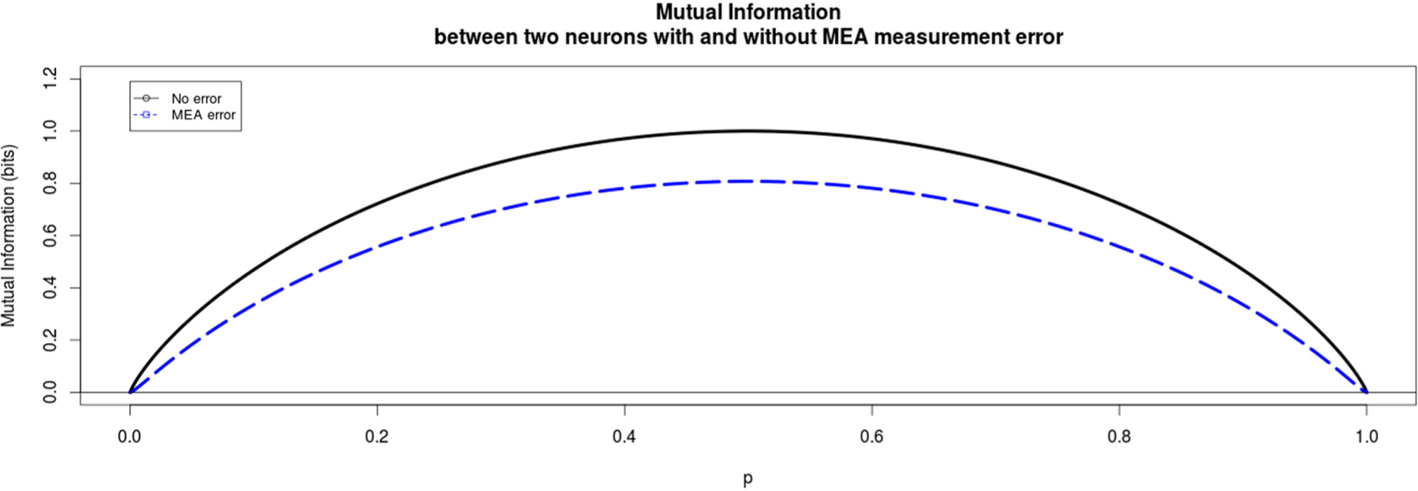
The induced error for each experimental method is modeled in a simplistic way that still reflects the main, qualitative differences of the two methods. In the following Figures 2 and 3 the qualitative difference between these two methods is presented clearly. For MEA data we find that the mutual information between the two neurons always decreases due to the miss-assignment, regardless of the parameter values we choose. In this particular plot in Figure 2 the conditional probabilities q0=0.2 and q0=0.9 and the probabilities of assigning a wrong spike to a neuron were ε=0.05 and δ=0.05 for the first and second neuron respectively. This trend was seen for all values of the conditional probabilities as well as the miss-assigning probabilities with the extreme case of ε=δ=0, where of course the mutual information did not decrease.
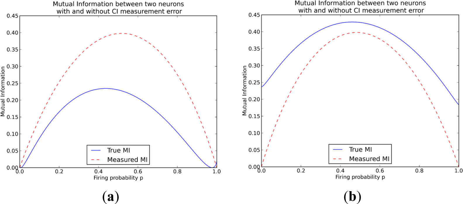
On the other hand when examining the difference in mutual information for the measurements from the CI data, the results are more complicated. The measured mutual information can either be less than the true mutual information, as is also the case for the MEA method, but it can also be higher than the true mutual information, meaning that using calcium imaging can lead to overestimating mutual information (Figure 3). The measured mutual information increases when q1 > q0 while it decreases when q1 < q0. The intuition is that the measurement moves probability mass from the unordered states (0,1 and 1,0) to the “both-firing” state (1,1). This can be seen easily in the following example: if a double spike (11,0) occurs it becomes a single (1,0)-measurement at the coarse-grained time-scale, while it should have become two (1,0)-measurements at a finer time-scale. For q1 > q0 most probability mass is already assigned to the state of both neurons firing (1,1), so the measurement lets the probabilities further diverge, increasing the mutual information. For the converse case the probabilities move closer to the equipartition, decreasing mutual information.
4. Discussion & Conclusions
Collaboration between experimental and theoretical neuroscientists is yielding more and more results. While both have their own expert knowledge, it is very valuable to bridge the gap between the two disciplines. It is important that theorists are aware of the opportunities and shortcomings of available experimental techniques, while experimentalists need to gain insight into what their data can and cannot be used for. Not only is the collaboration relevant for the validation of developing information theory to better understand complex systems, in return applying novel information-theoretical tools to neural networks can have clear benefits for understanding neural pathologies. Changes in the neural network structure, the impact of which is poorly understood, occurs in schizophrenic [47,48] and epileptic brains [49].
From the experimental point of view we demonstrate how the MEA and CI techniques can be used to record neural microcircuits simultaneously with neural dynamics. We also reviewed other popular techniques such as fMRI and EEG, which lack the spatial and/or temporal resolution to measure individual cells.
From the information-theoretical point of view we perform a numerical study in order to quantify and compare qualitatively the effects of the two techniques. Our results show that, while CI and MEA are both capable of measuring topology and dynamics of a neuronal network simultaneously, MEA consistently underestimates mutual information while CI may either underestimate or overestimate it (add spurious information). Also the dependence of the measurement effect as function of the firing probabilities appears qualitatively different. In conclusion, at least two experimental techniques for validating information-theoretical measures on neural microcircuits exist and are feasible, nevertheless the choice for either CI of MEA must be a careful one depending on experimental settings and the goal of the study.
While at the time of writing, only CI and MEAs satisfy our criteria for use with IT, the limits of these and other techniques are being developed further. Work is being done to combine the ideal temporal resolution of intracellular recording with the mass recording quality of MEA [43]. CI will profit from higher signal to noise ratios and cell specificity, among other things.
Acknowledgments
Rick Quax acknowledges the financial support of the Future and Emerging Technologies (FET) programme within the Seventh Framework Programme (FP7) for Research of the European Commission, under the FET-Proactive grant agreement TOPDRIM, number FP7-ICT-318121. Rick Quax and Omri Har-Shemesh acknowledge the financial support of the Future and Emerging Technologies (FET) programme within the Seventh Framework Programme (FP7) for Research of the European Commission, under the FET-Proactive grant agreement Sophocles, number FP7-ICT-317534. Carlos P. Fitzsimons is financed by the NWO VIDI grant H64.09.016.
PACS Codes: 87.19.lj; 89.70.Cf; 87.19.lo
Author Contributions
Rick Quax and Carlos P. Fitzsimons conceived and managed the project. Thijs I. Jung studied the literature on experimental techniques. Filippos Vogiatzian and Omri Har-Shemesh performed the numerical study of measurement errors. Rick Quax, Carlos P. Fitzsimons, Thijs I. Jung, Filippos Vogiatzian and Omri Har-Shemesh wrote the article. All authors have read and approved the final manuscript.
Conflicts of Interest
The authors declare no conflict of interest.
References
- Penrose, R.; Zenil, H.A. Computable Universe: Understanding and Exploring Nature as Computation; World Scientific: Singapore, Singapore, 2012. [Google Scholar]
- Crutchfield, J.P.; Feldman, D.P. Regularities unseen, randomness observed: Levels of entropy convergence. Chaos 2003, 13, 25–54. [Google Scholar]
- Crutchfield, J.P.; Ellison, C.J.; Mahoney, J.R. Time’s barbed arrow: Irreversibility, crypticity, and stored information. Phys. Rev. Lett. 2009, 103. [Google Scholar] [CrossRef]
- Williams, P.L.; Beer, R.D. Nonnegative decomposition of multivariate information 2010, arXiv, 1004.2515.
- Quax, R.; Apolloni, A.; Sloot, P.M.A. Information processing reveals how microscopic components affect the macroscopic system-state in complex networks 2011, arXiv, 1111.5483.
- James, R.G.; Ellison, C.J.; Crutchfield, J.P. Anatomy of a bit: Information in a time series observation. Chaos Interdiscip. J. Nonlinear Sci. 2011, 21. [Google Scholar] [CrossRef]
- Sloot, P.; Quax, R. Information processing as a paradigm to model and simulate complex systems. J. Comput. Sci. 2012, 3, 247–249. [Google Scholar]
- Lizier, J.T. The Local Information Dynamics of Distributed Computation in Complex Systems; Springer: Berlin, Germany, 2012. [Google Scholar]
- Bertschinger, N.; Rauh, J.; Olbrich, E.; Jost, J. Shared information—New insights and problems in decomposing information in complex systems, Proceedings of the European Conference on Complex Systems 2012, Brussels, Belgium, 3–7 September 2012; pp. 251–269.
- Griffith, V.; Chong, E.K.P.; James, R.G.; Ellison, C.J.; Crutchfield, J.P. Intersection information based on common randomness. Entropy 2014, 16, 1985–2000. [Google Scholar]
- Beer, R.D.; Williams, P.L. Information processing and dynamics in minimally cognitive agents. Cogn. Sci. 2014. [Google Scholar] [CrossRef]
- Shannon, C.E.; Weaver, W. Mathematical Theory of Communication; University of Illinois Press: Urbana, OH, USA, 1963. [Google Scholar]
- Cover, T.M.; Thomas, J.A. Elements of Information Theory; John Wiley & Sons: New York, NY, USA, 1991. [Google Scholar]
- Quax, R.; Apolloni, A.; Sloot, P.M. The diminishing role of hubs in dynamical processes on complex networks. J. R. Soc. Interface 2013, 10. [Google Scholar] [CrossRef]
- Lizier, J.T.; Prokopenko, M.; Zomaya, A.Y. Information modification and particle collisions in distributed computation. Chaos Interdiscip. J. Nonlinear Sci. 2010, 20. [Google Scholar] [CrossRef]
- Lizier, J.T.; Prokopenko, M.; Zomaya, A.Y. The information dynamics of phase transitions in random Boolean networks, Proceedings of Eleventh International Conference on the Simulation and Synthesis of Living Systems (Artificial Life XI), Winchester, UK, 5–8 August 2008; pp. 374–381.
- Barnett, L.; Lizier, J.T.; Harré, M.; Seth, A.K.; Bossomaier, T. Information flow in a kinetic Ising model peaks in the disordered phase. Phys. Rev. Lett. 2013, 111. [Google Scholar] [CrossRef]
- Lizier, J.T.; Flecker, B.; Williams, P.L. Towards a synergy-based approach to measuring information modification, Proceedings of 2013 IEEE Symposium on Artificial Life (ALife 2013), Singapore, Singapore, 16–19 April 2013; pp. 43–51.
- Schreiber, T. Measuring information transfer. Phys. Rev. Lett. 2000, 85. [Google Scholar] [CrossRef]
- Lizier, J.T.; Prokopenko, M.; Zomaya, A.Y. Local information transfer as a spatiotemporal filter for complex systems. Phys. Rev. E 2008, 77. [Google Scholar] [CrossRef]
- Quax, R.; Kandhai, D.; Sloot, P.M. Information dissipation as an early-warning signal for the Lehman Brothers collapse in financial time series. Sci. Rep. 2013, 3. [Google Scholar] [CrossRef]
- Bullmore, E.; Sporns, O. Complex brain networks: Graph theoretical analysis of structural and functional systems. Nat. Rev. Neurosci. 2009, 10, 186–198. [Google Scholar]
- Markram, H.; Lubke, J.; Frotscher, M.; Roth, A.; Sakmann, B. Physiology and anatomy of synaptic connections between thick tufted pyramidal neurones in the developing rat neocortex. J. Physiol. 1997, 500, 409–440. [Google Scholar]
- Smetters, D.; Majewska, A.; Yuste, R. Detecting action potentials in neuronal populations with calcium imaging. Methods 1999, 18, 215–221. [Google Scholar]
- Stosiek, C.; Garaschuk, O.; Holthoff, K.; Konnerth, A. In vivo two-photon calcium imaging of neuronal networks. Proc. Natl. Acad. Sci. 2003, 100, 7319–7324. [Google Scholar]
- Dreosti, E.; Lagnado, L. Optical reporters of synaptic activity in neural circuits. Exp. Physiol. 2011, 96, 4–12. [Google Scholar]
- Grewe, B.F.; Langer, D.; Kasper, H.; Kampa, B.M.; Helmchen, F. High-speed in vivo calcium imaging reveals neuronal network activity with near-millisecond precision. Nat. Methods 2010, 7, 399–405. [Google Scholar]
- Gobel, W.; Helmchen, F. In vivo calcium imaging of neural network function. Physiology 2007, 22, 358–365. [Google Scholar]
- Garaschuk, O.; Milos, R.-I.; Grienberger, C.; Marandi, N.; Adelsberger, H.; Konnerth, A. Optical monitoring of brain function in vivo: From neurons to networks. Pflüg. Arch. 2006, 453, 385–396. [Google Scholar]
- Luo, L.; Callaway, E.M.; Svoboda, K. Genetic dissection of neural circuits. Neuron 2008, 57, 634–660. [Google Scholar]
- Giordano, G.; Costa, L.G. Primary neurons in culture and neuronal cell lines for in vitro neurotoxicological studies. Methods Mol. Biol. 2011, 758, 13–27. [Google Scholar]
- Marshel, J.H.; Deisseroth, K. Genetically encoded voltage sensor goes live. Nat. Biotechnol. 2013, 31, 994–995. [Google Scholar]
- Chen, T.-W.; Wardill, T.J.; Sun, Y.; Pulver, S.R.; Renninger, S.L.; Baohan, A.; Schreiter, E.R.; Kerr, R.A.; Orger, M.B.; Jayaraman, V.; et al. Ultrasensitive fluorescent proteins for imaging neuronal activity. Nature 2013, 499, 295–300. [Google Scholar]
- Stetter, O.; Battaglia, D.; Soriano, J.; Geisel, T. Model-free reconstruction of excitatory neuronal connectivity from calcium imaging signals. Comput. Biol. 2012, 8. [Google Scholar] [CrossRef]
- Cousin, M.A. Use of FM1-43 and other derivatives to investigate neuronal function. Curr. Protoc. Neurosci. 2008, 43. [Google Scholar] [CrossRef]
- James, C.D.; Spence, A.J.H.; Dowell-Mesfin, N.M.; Hussain, R.J.; Smith, K.L.; Craighead, H.G.; Isaacson, M.S.; Shain, W.; Turner, J.N. Extracellular recordings from patterned neuronal networks using planar microelectrode arrays. IEEE Trans. Biomed. Eng. 2004, 51, 1640–1648. [Google Scholar]
- Meister, M.; Pine, J.; Baylor, D.A. Multi-neuronal signals from the retina: Acquisition and analysis. J. Neurosci. Methods 1994, 51, 95–106. [Google Scholar]
- Frega, M.; Tedesco, M.; Massobrio, P.; Pesce, M.; Martinoia, S. Network dynamics of 3D engineered neuronal cultures: A new experimental model for in-vitro electrophysiology. Sci. Rep. 2014, 30. [Google Scholar] [CrossRef]
- Einevoll, G.T.; Franke, F.; Hagen, E.; Pouzat, C.; Harris, K.D. Towards reliable spike-train recordings from thousands of neurons with multielectrodes. Curr. Opin. Neurobiol. 2012, 22, 11–17. [Google Scholar]
- Quiroga, R.Q. Spike sorting. Curr. Biol. 2012, 22, 45–46. [Google Scholar]
- Quiroga, R.Q.; Panzeri, S. Extracting information from neuronal populations: Information theory and decoding approaches. Nat. Rev. Neurosci. 2009, 10, 173–185. [Google Scholar]
- Cheung, K.C.; Renaud, P.; Tanila, H.; Djupsund, K. Flexible polyimide microelectrode array for in vivo recordings and current source density analysis. Biosens. Bioelectron. 2007, 22, 1783–1790. [Google Scholar]
- Spira, M.E.; Hai, A. Multi-electrode array technologies for neuroscience and cardiology. Nat. Nanotechnol. 2013, 8, 83–94. [Google Scholar]
- Cossart, R.; Ikegaya, Y.; Yuste, R. Calcium imaging of cortical networks dynamics. Cell Calcium 2005, 37, 451–457. [Google Scholar]
- Reichinnek, S.; von Kameke, A.; Hagenston, A.M.; Freitag, E.; Roth, F.C.; Bading, H.; Hasand, M.T.; Draguhna, A.; Both, M. Reliable optical detection of coherent neuronal activity in fast oscillating networks in vitro. NeuroImage 2012, 60, 139–152. [Google Scholar]
- Harris, K.D.; Henze, D.A.; Csicsvari, J.; Hirase, H.; Buzsáki, G. Accuracy of tetrode spike separation as determined by simultaneous intracellular and extracellular measurements. J. Neurophysiol. 2000, 84, 401–414. [Google Scholar]
- Kim, D.-J.; Kent, J.S.; Bolbecker, A.R.; Sporns, O.; Cheng, H.; Newman, S.D.; Puce, A.; O’Donnell, B.F.; Hetrick, W.P. Disrupted modular architecture of cerebellum in schizophrenia: A graph theoretic analysis. Schizophr. Bull. 2014, 40. [Google Scholar] [CrossRef]
- Shim, M.; Kim, D.-W.; Lee, S.-H.; Im, C.-H. Disruptions in small-world cortical functional connectivity network during an auditory oddball paradigm task in patients with schizophrenia. Schizophr. Res. 2014, 156, 197–203. [Google Scholar]
- Da Silva, F.H.L.; Gorter, J.A.; Wadman, W.J. Epilepsy as a dynamic disease of neuronal networks. Handb. Clin. Neurol. 2012, 107, 35–62. [Google Scholar]

| CI | MEA | |
|---|---|---|
| Temporal resolution | Can distinguish spikes spaced 40–50 ms apart | Nearly instant, can distinguish spikes spaced ~1 ms apart |
| Spatial resolution | Individual neurons | Extracellular electrodes are spaced according to the need of the user (50–250 μm is often used) and may measure individual neurons dependent on placement of the array and spike sorting software |
| Temporal challenge | Onset-lag, decay lag | None |
| Spatial challenge | None | Spikes are assigned to neurons by offline inference |
| Invasiveness | Neurons: none, animals: yes | Neurons: none, animals: yes |
| Numbers of cells measured | ~1501 | ~2001 |
| Cell specificity? | No, only with genetic dyes | No |
| Blind to | Non-active cells | Non-active cells & sub threshold fluctuations |
1The number of cells that are being measured depends on various variables (e.g., which type of MEA is used or on how big is the area where CI is done). The numbers listed here are a maximum estimation.
© 2014 by the authors; licensee MDPI, Basel, Switzerland This article is an open access article distributed under the terms and conditions of the Creative Commons Attribution license (http://creativecommons.org/licenses/by/4.0/).
Share and Cite
Jung, T.I.; Vogiatzian, F.; Har-Shemesh, O.; Fitzsimons, C.P.; Quax, R. Applying Information Theory to Neuronal Networks: From Theory to Experiments. Entropy 2014, 16, 5721-5737. https://doi.org/10.3390/e16115721
Jung TI, Vogiatzian F, Har-Shemesh O, Fitzsimons CP, Quax R. Applying Information Theory to Neuronal Networks: From Theory to Experiments. Entropy. 2014; 16(11):5721-5737. https://doi.org/10.3390/e16115721
Chicago/Turabian StyleJung, Thijs I., Filippos Vogiatzian, Omri Har-Shemesh, Carlos P. Fitzsimons, and Rick Quax. 2014. "Applying Information Theory to Neuronal Networks: From Theory to Experiments" Entropy 16, no. 11: 5721-5737. https://doi.org/10.3390/e16115721