Markov State Models for Rare Events in Molecular Dynamics

Abstract
: Rare, but important, transition events between long-lived states are a key feature of many molecular systems. In many cases, the computation of rare event statistics by direct molecular dynamics (MD) simulations is infeasible, even on the most powerful computers, because of the immensely long simulation timescales needed. Recently, a technique for spatial discretization of the molecular state space designed to help overcome such problems, so-called Markov State Models (MSMs), has attracted a lot of attention. We review the theoretical background and algorithmic realization of MSMs and illustrate their use by some numerical examples. Furthermore, we introduce a novel approach to using MSMs for the efficient solution of optimal control problems that appear in applications where one desires to optimize molecular properties by means of external controls.1. Introduction
Stochastic processes are widely used to model physical, chemical or biological systems. The goal is to approximately compute interesting properties of the system by analyzing the stochastic model. As soon as randomness is involved, there are mainly two options for performing this analysis: (1) Direct sampling and (2) the construction of a discrete coarse-grained model of the system. In a direct sampling approach, one tries to generate a statistically significant amount of events that characterize the property of the system one in which is interested. For this purpose, computer simulations of the model are a powerful tool. For example, an event could refer to the transition between two well-defined macroscopic states of the system. In chemical applications, such transitions can often be interpreted as reactions or, in the context of a molecular system, as conformational changes. Interesting properties are, e.g., average waiting times for such reactions or conformational changes and along which pathways the transitions typically occur. The problem with a direct sampling approach is that many interesting events are so-called rare events. Therefore, the computational effort for generating sufficient statistics for reliable estimates is very high, and particularly if the state space is continuous and high dimensional, estimation by direct numerical simulation is infeasible.
Available techniques for rare event simulations in continuous state space are discussed in [1]. In this article, we will discuss approach (2) to the estimation of rare event statistics via discretization of the state space of the system under consideration. That is, instead of dealing with the computation of rare events for the original, continuous process, we will approximate them by a so-called Markov State Model (MSM) with discrete finite state space. The reason is that for such a discrete model, one can numerically compute many interesting properties without simulation, mostly by solving linear systems of equations as in discrete transition path theory (TPT) [2]. We will see that this approach, called Markov State Modeling, avoids the combinatorial explosion of the number of discretization elements with the increasing size of the molecular system in contrast to other methods for spatial discretization.
The actual construction of an MSM requires one to sample certain transition probabilities of the underlying dynamics between sets. The idea is: (1) to choose the sets such that the sampling effort is much lower than the direct estimation of the rare events under consideration; and (2) to compute all interesting quantities for the MSM from its transition matrix, cf. [2,3]. There are many examples for the successful application of this strategy. In [4], for example, it was used to compute dominant folding pathways for the PinWW domain in explicit solvent. However, we have to make sure that the Markov State Model approximates the original dynamics well enough. For example, the MSM should correctly reproduce the timescales of the processes of interest. These approximation issues have been discussed since more than a decade now [5,6]; in this article, we will review the present state of research on this topic. In the algorithmic realization of Markov State Modeling for realistic molecular systems, the transition probabilities and the respective statistical uncertainties are estimated from short molecular dynamics (MD) trajectories only, cf.[7]. This makes Markov State Modeling applicable to many different molecular systems and processes, cf.[8–13].
In the first part of this article, we will discuss the approximation quality of two different types of Markov State Models that are defined with respect to a full partition of state space or with respect to so-called core sets. We will also discuss the algorithmic realization of MSMs and provide references to the manifold of realistic applications to molecular systems in equilibrium that are available in the literature today.
The second part will show how to use MSMs for optimizing particular molecular properties. In this type of application, one wants to steer the molecular system at hand by external controls in a way such that a pre-selected molecular property is optimized (minimized or maximized). That is, one wants to compute a specific external control from a family of admissible controls that optimizes the property of interest under certain side conditions. The property to be optimized can be quite diverse: For example, it can be (1) the population of a certain conformation that one wants to maximize under a side condition that limits the total work done by the external control or (2) the mean first passage time to a certain conformation that one wants to minimize (in order to speed up a rare event), but under the condition that one can still safely estimate the mean first passage time of the uncontrolled system. The theoretical background of case (1) has been considered in [14], for example, and of case (2) in [1,15]. There, one finds the mathematical problem that has to be solved in order to compute the optimal control. Here, we will demonstrate that one can use MSMs for the efficient solution of such a mathematical problem (for both cases). We will see that the spatial discretization underlying an MSM turns the high-dimensional continuous optimal control problem into a rather low-dimensional discrete optimal control problem of the same form that can be solved efficiently. Based on these insights, MSM discretization yields an efficient algorithm for solving the optimal control problem, whose performance we will outline in some numerical examples, including an application to alanine dipeptide.
2. MSM Construction
Let (Xt)t≥0 be a time-continuous Markov process on a continuous state space, E, e.g., E ⊂ Rd. That is, Xt is the state of the molecular system at time t resulting from any usually used form of molecular dynamics simulation, be it based on Newtonian dynamics with thermostats or resulting from Langevin dynamics or other diffusion molecular dynamics models. The idea of Markov State Modeling is to derive a Markov chain, (X̂k)k∈ℕ, on a finite and preferably small state space Ê = {1, ..., n} that models characteristic dynamics of the continuous process, (Xt). For example, in molecular dynamics applications, such characteristic dynamics could refer to protein folding processes [16,17], conformational rearrangements between native protein substates [18,19], or ligand binding processes [20]. Since the approximating Markov chain, (Xk)k∈ℕ, lives on a finite state space, the construction of an MSM boils down to the computation of its transition matrix, P:
The main benefit is that for a finite Markov chain, one can compute many interesting dynamical properties directly from its transition matrix, e.g., timescales and the metastability in the system [5,21,22], a hierarchy of important transition pathways [2] or mean first passage times between selected states. With respect to an MSM, these computations should be used afterwards to answer related questions for the original continuous process. To do this, we must be able to link the states of the Markov chain back to the spatial information of the original process, and the approximation of the process (Xt) by the MSM must be valid in some sense.
Having this in mind, the first natural idea is to let the states of an MSM correspond to sets A1, ..., An ⊂ E in continuous state space that form a full partition, i.e.:
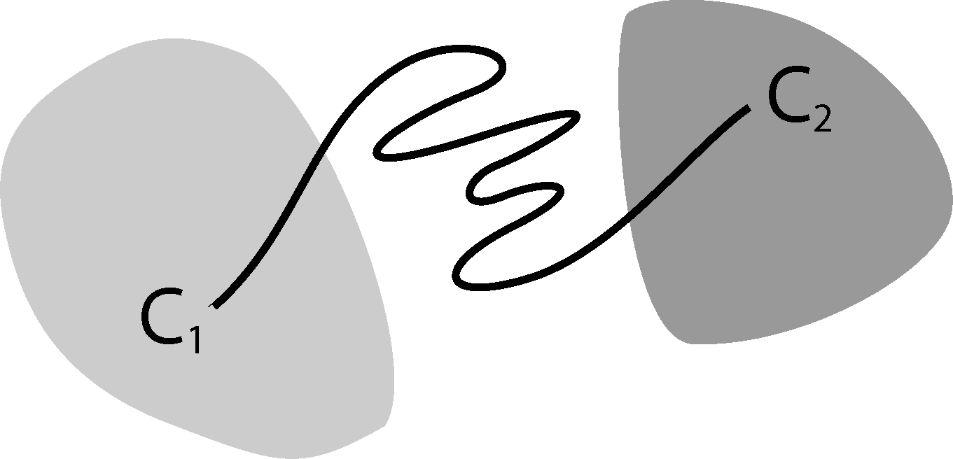
It is well known that this process is not Markovian, mainly due to the so-called recrossing problem. This refers to the fact that the original process typically crosses the boundary between two sets, Ai and Aj, several times when transitions take place, as illustrated in Figure 1. This results in cumulative transitions between indices i and j for the index process, that is, a not memoryless transition behavior.
The non-Markovianity of the index process is often seen as a problem in Markov State Modeling, because many arguments assume that X̃k is a Markov process. In this article, we will not make this assumption. We interpret the process (X̃k) as a tool to construct the following transition matrix, Pτ:
3. Analytical Results
In order to compare the MSM to the continuous process, we introduce one of the key objects for our analysis, the transfer operator of a Markov process. We assume that the Markov process (Xt) has a unique, positive invariant probability measure, μ, and that it is time-reversible. Then, for any time-step, t ≥ 0, we define the transfer operator, Tt, via the property:
Note that Tt is nothing else other than the propagator of densities under the dynamics, but the densities are understood as densities with respect to the measure, μ. That is, if the Markov process is initially distributed according to:
The benefit of working with μ-weighted densities is that the transfer operator, Tt, becomes essentially self-adjoint on L2(μ) for all cases of molecular dynamics satisfying some form of detailed balance condition. Hence, it has real eigenvalues and orthogonal eigenvectors with respect to Equation (7) (or, at least, the dominant spectral elements are real-valued). Moreover, the construction of an MSM can be seen as a projection of the transfer operator [25]. Assume Q is an orthogonal projection in L2(μ) onto an n-dimensional subspace, D ⊂ L2(μ), with 𝟙 ∈ D, and χ1, ..., χn is a basis of D. Then, the so-called projected transfer operator, QTτQ: D → D, has the matrix representation:
Full Partition MSM. If we choose χi = 𝟙Ai to be the characteristic function of set Ai for i = 1, ..., n, one can easily check that we get M = I to be the identity matrix and:
The previously constructed transition matrix of the MSM based on a full partition can be interpreted as a projection onto a space of densities that are constant on the partitioning sets. This interpretation of an MSM is useful, since it allows one to analyze its approximation quality. For example, in [25,26], it is proven that we can reproduce an eigenvalue, λ, of a self-adjoint transfer operator, Tt, by the MSM by choosing the subspace appropriately. That is, if u is a corresponding normalized eigenvector, Q the orthogonal projection to a subspace, D, with 𝟙 ∈ D, then there exists an eigenvalue, λ̂, of the projected transfer operator, QTtQ, with:
In particular, for , one can simplify the equation to:
An eigenvalue, λi, of the transfer operator directly relates to an implied timescale, i, of the system via:
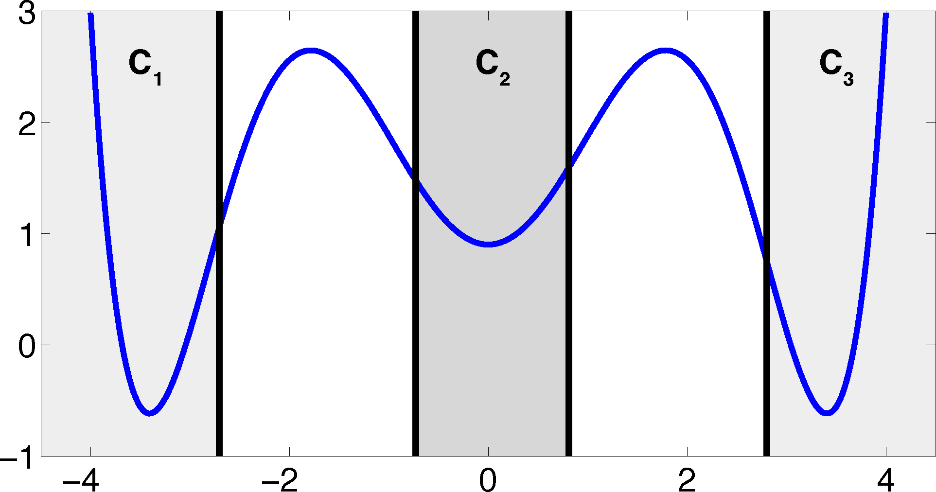
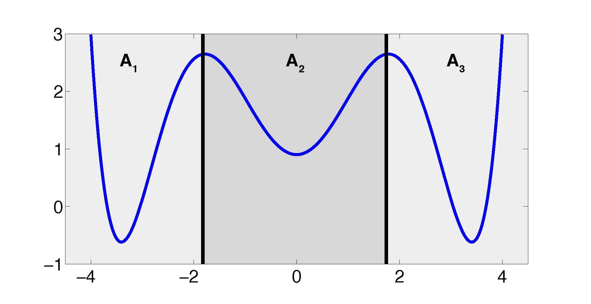
The projection error, δ, depends on our choice of the discretizing sets. As an example, let us consider a diffusion in the potential that is illustrated in Figure 2, that is, the reversible Markov process given by the stochastic differential equation:
The figure also shows a choice of three sets that form a full partition of state space. The computation of the transition matrix Equation (4) for σ = 0.7 and a lag time τ = 1 yields:
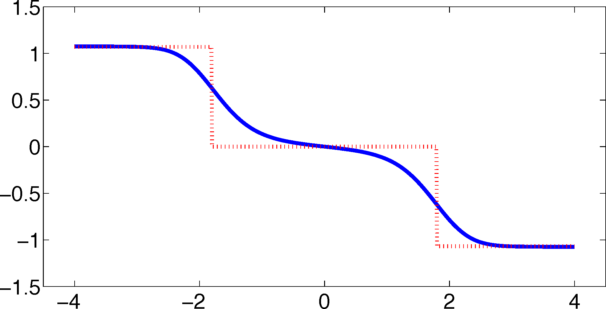
As one can see, the timescales are strongly underestimated. This is a typical phenomenon. From a statistical point of view, the recrossing problem will lead to cumulatively appearing transition counts when one computes the transition probabilities, ℙμ[Xτ ∈ Aj|X0 ∈ Ai], from a trajectory (Xt), as discussed above. Therefore, on average, transitions between sets seem to become too likely, and hence, the processes in the coarse-grained system get accelerated. We have seen in Equation (14) that this cannot happen if the associated eigenvectors can be approximated well by the subspace that corresponds to the MSM. Figure 3 shows the first non-trivial eigenvector, u1, belonging to the timescale T1 = 103.7608 and its best-approximation by a step function.
The eigenvector is indeed almost constant in the vicinity of the wells, but within the transition region between the wells, the eigenvector is varying and the approximation by a step function is not accurate. Therefore, we have two explanations of why the main error is introduced in the region close to shared boundaries of neighboring sets: (1) because of recrossing issues; and (2) because of the main projection error of the associated eigenvector. Of course, one solution would be an adaptive refinement of the discretization, that is, one could choose a larger number of smaller sets, such that the eigenvector is better approximated by a step function on these sets. In the following section, we will present an alternative solution for overcoming the recrossing problem and reducing the projection error without refining the discretization.
4. The Core Set Approach
From Equation (10), we know how to compute a matrix representation for a projected transfer operator for an arbitrary subspace, D ⊂ L2(μ). For a given basis, χ1, ..., χn, we have to compute Equations (11) and (12), so:
Now, the question is if there is another basis other than characteristic functions that: (a) is more adapted to the eigenvectors of the transfer operator; and (b) still leads to a probabilistic interpretation of the matrix entries Equation (17), such that scalar products never have to be computed. The basic idea is to stick to a set-oriented definition of the basis, but to relax the full partition constraint. We will define our basis with respect to so-called core sets, C1, ..., Cn ⊂ E, that are still disjoint, so Ci ∩ Cj = ∅, but they do not have to form a full partition. Figure 4 suggests that this could lead to a reduction of the recrossing phenomenon, since the sets do not share boundaries anymore.
Now, we use the core sets to define our basis functions, χ1, ..., χn. Assume Tτ is, again, a self-adjoint transfer operator and consider n core sets C1, ..., Cn. For every i, take the committor function, χi, of the process with respect to core set Ci; that is, χi(x) denotes the probability to hit the core set, Ci, next, rather than the other core sets, when starting the process in x. If we now study the projection, Q, onto the space spanned by these committor functions, the two following properties hold [25,27].
- (P1)
The matrices, M and P, in Equation (10) can be written as:
where ( ) and ( ) are forward and backward milestoning processes [25,28]; that is, if the process came at time t = kτ, last from core set Ci and if the process went next to core set Cj after time t = kτ.- (P2)
Let ui be an eigenvector of Tτ that is almost constant on the core sets. Let the region C = E\∪iCi that is not assigned to a core set be left quickly enough, so 𝔼x[τ(Cc)] ≪ i for all x ∈ C, where i is the timescale associated with ui and 𝔼x[τ(Cc)] is the expected hitting time of Cc = ∪iCi when starting in x ∈ C. Then, ‖ui − Qui‖ is small; so, the committor approximation to the eigenvector is accurate.
The message behind (P1) is that it is possible to relax the full partition constraint and use a core set discretization that does not cover the whole state space. We can still define a basis for a projection of the transfer operator that leads to a matrix representation that can be interpreted in terms of transition probabilities.
Important Remark: The construction of the projection onto the committors is only necessary for theoretical purposes. In practice, neither the committor functions nor scalar products between the committors have to be computed numerically, since the matrix entries of M and P can be estimated from trajectories again.
Property (P2) yields that the relaxation of the full partition constraint should also lead to an improvement of the MSM if the region, C, between the core sets is typically left on a faster timescale than the processes of interest taking place. Let us get back to the example from above. We will see that we can achieve a strong improvement of the approximation by simply excluding a small part of state space from our discretization. In Figure 5, we have turned our initial full partition into a core set discretization by removing parts of the transition region between the wells.
The matrix PQ = PM−1 that represents the projection, QTτ Q, of the transfer operator onto the committor space associated with the core sets is given by:
From the discussion above, this has to be expected, because the eigenvectors are almost constant in the vicinity of the wells, and we removed a part of state space from the discretization that is typically left quickly compared to the timescales, T1 and T2. Therefore, the committor functions should deliver a good approximation of the first two eigenvectors. Figure 6 underlines this theoretical result.
5. Practical Considerations and MD Applications
In the previous sections, we have interpreted the construction of an MSM as a projection of the dynamics onto some finite dimensional ansatz space. We have discussed two types of spaces that both have been defined on the basis of a set discretization. First, we chose a full partition of state space and the associated space of step functions, and second, we analyzed a discretization by core sets and the associated space spanned by committor functions. These two methods have the advantage that the resulting projections lead to transition matrices for the MSM with entries that are given in terms of transition probabilities between the sets. That is, one can compute estimates for the transition matrices from simulation data. This is an important property for practical applications, because it means that we never need to compute committor functions or scalar products between committors or step functions. We rather generate trajectories x0,x1, ...xN of the process (Xt), let us say, for a time step h > 0, so xi = Xhi. For example, we can then define for a full partition, A1, ..., Am, and a lag time τ = nh the discrete trajectory sk = i ⇔ xk ∈ Ai and compute the matrix, P̂:
Since, in practice, we will only have a finite amount of data available, we will have statistical errors when constructing an MSM. This is an additional error to the projection error related to the discretization that we have discussed above. On the other hand, one should note that these errors are not independent of each other. For example, it is clear that if we take a full partition of state space, and we let the partition become arbitrarily fine by letting the number of sets go to infinity, the discretization error will vanish. At the same time, for a fixed amount of statistics, the statistical error will become arbitrarily large, because we will need to compute more and more estimators for transition events between the increasing number of sets. For more information on statistical errors, we refer to the literature [7,29].
Besides the choice of discretization and the available statistics, the estimates above also depend on a lag time, τ. This dependence can be used to validate an MSM by a Chapman–Kolmogorov test [7]. This is based on the fact that the MSM matrices approximately form a semi-group for all large enough lag times τ > τ*; although, for small lag times, this is typically not true, due to memory effects. These facts also motivate one to look at something, like an infinitesimal generator, that approximately generates these MSM transition matrices for large enough lag times. In [27], two types of generator constructions have been compared for a core set setting. The first generator, K, is simply constructed from the transition rates between the core sets in the milestoning sense, that is:
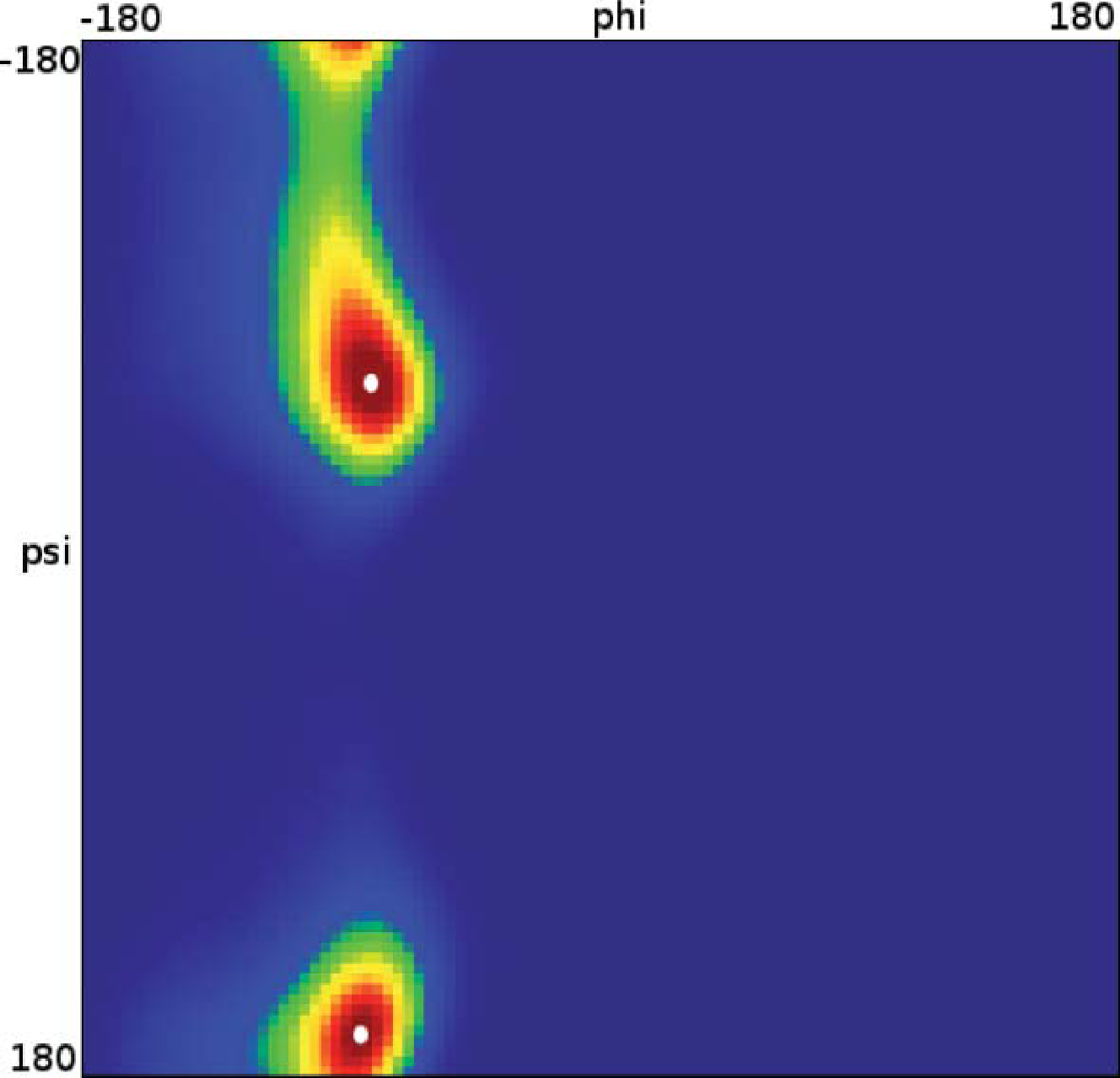
Let us now analyze how the choice of core sets, particularly the size of the core sets, influences the resulting approximation. Therefore, we consider an MD example that was discussed in [27], namely one molecule of alanine dipeptide monitored via its ϕ and ψ backbone dihedral angles. Two core sets are defined as balls with radius r around the two points with angular coordinates xα = (−80, −60) and xβ = (−80, 170). The stationary distribution of the process and the two centers of the core sets, xα,xβ, in the angular space are shown in Figure 7.
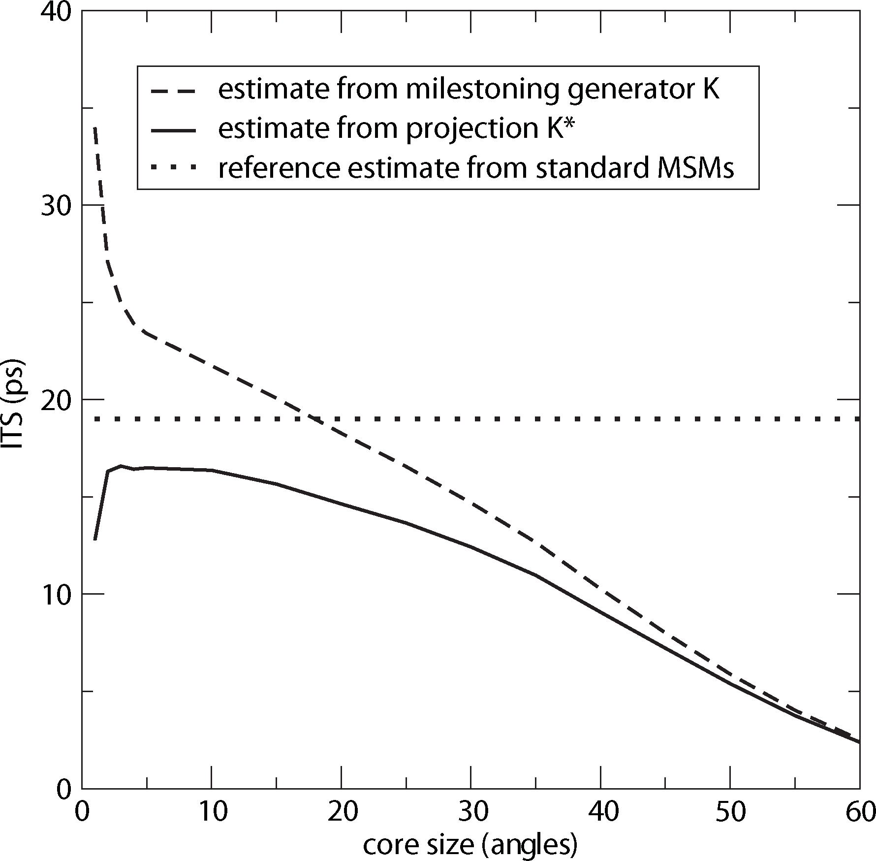
For computing a reference timescale, several MSMs based on three different full partitions using 10, 15 and 250 sets have been constructed for increasing lag times. In [27], it is shown that in each setting, the estimate for the longest implied timescale of the process converged to ≈19 ps for large enough τ. Now, the implied timescales for the two different generators, K Equation (22) and K* Equation (23), are computed. In Figure 8, the resulting timescales are plotted against the reference timescale ≈ 19 ps for varying size of the core sets.
One can see that the estimate by the milestoning generator, K, is rather sensitive to the size of core sets. It overestimates the timescales for small core sizes and underestimates it for larger core sizes. On the other hand, the projected generator, K*, can never overestimate the timescale, due to its interpretation as projection. It is also rather robust against the choice of size of the core sets until the core sets become too large, e.g., r > 15. Then, the discretization becomes close to a full partition discretization using only two sets. In this case, the timescales have to be underestimated heavily, because of recrossing phenomena. On the other hand, the underestimation for very small core sets has to be explained by a lack of statistics. When the core sets are chosen as arbitrarily small, it is clearly more difficult for the process to hit the sets, and therefore, transition events become rare. Note that for the straightforward milestoning generator, K, the processes seem to become very slow, but for the projected generator K* = KM−1, this effect is theoretically corrected by the mass matrix, M. Nevertheless, in both cases, the generation of enough statistics will be problematic for too small core sets.
6. Further Applications in MD
Markov State Modeling has been show to apply successfully to many different molecular systems, like peptides, including time-resolved spectroscopic experiments [10–12], proteins and protein folding [4,9,13], DNA [31] and ligand-receptor interaction [32]. In most of the respective publications, full partition MSMs are used, and the underlying discretization is based on cluster finding methods (see [7] for a review), while the sampling issues are tackled by means of ideas from enhanced sampling [33] and based on ensembles of rather short trajectories instead of one long one, cf.[4]. Core set-based approaches have been used just recently [10,27]; related algorithms are less well developed. However, recent work has shown that and how every full partition MSM can be easily transformed into a core set-based MSM with significantly improved approximation quality [34], making core set MSMs the most promising next generation MSM tools.
Very Rare Transitions between Discretization Sets. When constructing a full partition or a core set MSM, we have to estimate transition probabilities between sets in state space, and it can happen that we cannot avoid that some of these transitions are very rare. That is, the transition probabilities for a lag time, τ, between some sets can be non-zero, but small even, if compared to the remaining transition probabilities that are small already. This is why it is important to note that neglecting these very rare transitions during the construction of an MSM does not harm its approximation quality. For example, we can define for a transition matrix, P, another transition matrix, P̃, by:
Computation from Trajectories. Clearly, constructing and analyzing a core set MSM will only have a computational advantage compared to the direct sampling of a rare event if the transition events between neighboring core sets occur on a much shorter timescale than the rare event itself. One should note that from the purely theoretical point of view, it would be optimal to choose only very few core sets in the most metastable regions of state space, because this would minimize the projection error δ = ‖u − Qu‖ for each dominant eigenvector u, as discussed in Section 3. On the other hand, when estimating the MSM from trajectories, only a finite amount of statistics will be available, so there will also be a statistical error. In order to keep the total error small, additional core sets in less metastable parts of state space typically have to be introduced. In the end, this makes the estimation of a core set MSM possible without having to sample rare events. Note that the projection error is still under control, as long as there is a transition region between the core sets that is typically left very quickly (see Property (P2) in Section 4).
In practice, the statistics of the transition events between core sets will preferably be estimated from many short trajectories using milestoning techniques [27,28] and parallel computing. However, any algorithm for the construction of a core set MSM has to find a balance between sampling issues (not too many too long trajectories needed) and discretization issues (not too many core sets). Construction of such an algorithm still is ongoing research.
This article cannot give a detailed review on the algorithmic realization of MSMs for realistic molecular systems and on the findings resulting from such applications, since this is discussed to some extent elsewhere; see [7] for a recent review of the algorithmic aspects and [32,35] for ligand-receptor interaction.
7. MSM for Optimal Control Problems
In this section, we will borrow ideas from the previous section and explain how MSMs can be used to discretize optimal control problems that are linear-quadratic in the control variables and which appear in, e.g., the sampling of rare events. Specifically, we consider the case that (Xt)t≥0 is the solution of:
Other choices of f in Equation (26) result in alternative applications. One obvious application would be to set τ = T to a fixed time and f to the characteristic function of the complement of a conformation set C, f = 𝟙E\C. In this case, minimization of J wrt. the control ut would mean maximization of the probability to find the system in the conformation, C, until time T under a penalty on the external work done to the system. See [14] for more details on such applications.
There are other types of cost functions, J, one might consider, e.g., control until a deterministic finite time τ = T is reached or, even, τ → ∞, and the construction would follow analogously. For compactness, we consider here only cost functions as in Equation (27).
Optimal Control and Equilibrium Expectation Values. It turns out that when minimizing J, it is sufficient to consider control strategies that are Markovian and depend only on Xt, i.e., we consider feedback laws of the form ut = α(Xt) for some smooth function, α: E → ℝd. Moreover, only controls with finite energy are considered, for otherwise, J(u; x) = ∞. For control problems of the form Equations (26) and (27), the optimal feedback function can be shown to be α*(x) = − ∇W, where W is the value function or optimal-cost-to-go [1,15]:
The difficulty is that Equation (29) is a nonlinear partial differential equation and for realistic high-dimensional systems, it is not at all obvious how to discretize it, employing any kind of state space partitioning. It has been demonstrated in [14,15] that Equation (29) can be transformed into a linear equation by a logarithmic transformation. Setting: W (x) = −ε log ϕ(x) it readily follows, using chain rule and Equation (29), that ϕ solves the linear equation:
Remark. The optimization problem Equation (28) admits an interpretation in terms of entropy minimization: let and denote the path probability measures of controlled and uncontrolled trajectories starting at x at time t = 0, and set:
8. MSM Discretization of Optimal Control Problems
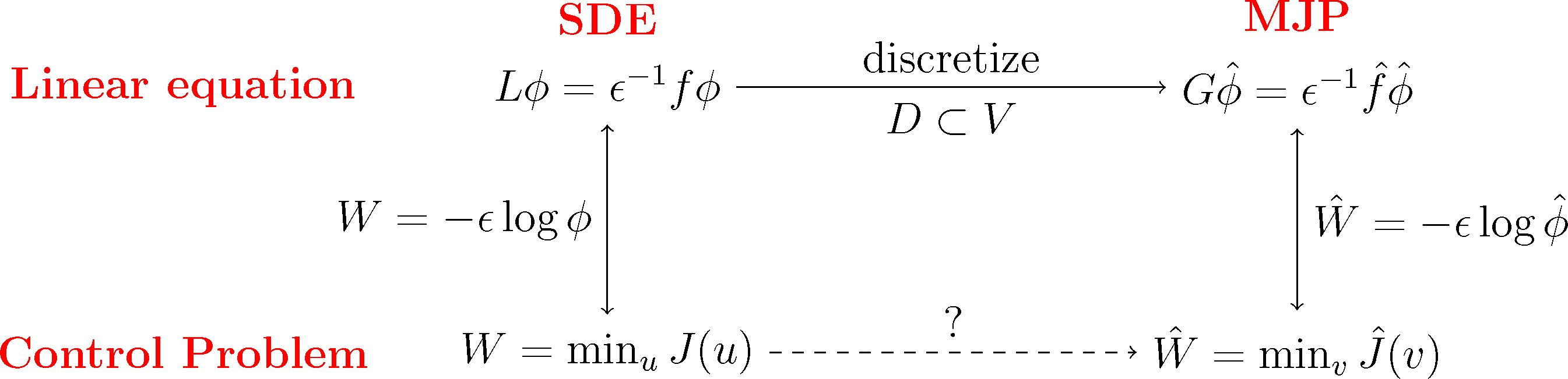
The basic idea is now to choose a subspace, D ⊂ L2(μ), with basis χ1,...,χn as in Markov State Modeling and then discretize the dynamic programming Equation (29) of our optimal control problem by projecting the equivalent log transformed Equation (31) onto that subspace. As we will see, the resulting discrete matrix equation can be transformed back into an optimal control problem for a discrete Markov jump process (MJP).
We will do this construction for the full partition case χi = 𝟙Ai and the core set case χi = qi discussed earlier. We will see that in both cases, we arrive at a structure-preserving discretization of the original optimal control problem, where the states of the corresponding MJP will be related to the partition subsets, Ai. The first case will give us back a well-known lattice discretization for continuous control problems, the Markov chain approximation [39]. This is illustrated in the following diagram:
Subspace Projection. The key step for the discretization is that we pick a suitable subspace, D ⊂ L2(μ), that is adapted to the boundary value problem Equation (31). Specifically, we require that the subspace contains the constant function, 𝟙 ∈ D, and that it gives a good representation of the most dominant metastable sets. To this end, we choose basis functions χ1,...,χn+1 with the following properties:
- (S1)
The χi form a partition of unity, that is .
- (S2)
The χi are adapted to the boundary conditions in Equation (31), that is χn+1|A = 1 and χi|A = 0 for i ∈ {1,...,n}.
Now, let Q be the orthogonal projection onto D, and define the matrices:
The best approximation error ‖Q⊥ϕ‖μ = infψ∈D‖ϕ − ψ‖μ, which appears in Equation (36), will vanish if the χi form an arbitrarily fine full partition of E. If we follow the core set idea from Section 4 and choose the χi to be committor functions, we have good control over ‖Q⊥ϕ‖μ. Due to [41]:
Properties of the Projected Problem. We introduce now the diagonal matrix, Λ, with entries Λii = ∑jFij (zero otherwise) and the full matrix G = K − ε−1(F − Λ), and rearrange Equation (34) as follows:
This equation can be given a stochastic interpretation. To this end, let us introduce the vector, π ∈ ℝn+1, with nonnegative entries πi = 〈χi, 𝟙〉 and notice that ∑iπi = 1 follows immediately from the fact that the basis functions, χi, form a partition of unity, i.e., ∑iχi =𝟙. This implies that π is a probability distribution on the discrete state space Ê = {1,...,n + 1}. We summarize properties of the matrices, K, F and G; see also [41]:
- (M1)
K is a generator matrix of an MJP (X̂t)t≥0 (i.e., K is a real-valued square matrix with row sum zero and positive off-diagonal entries) with stationary distribution, π, that satisfies detailed balance:
- (M2)
F ≥ 0 (entry-wise) with πiFij = πjFji for all i, j ∈ Ê.
- (M3)
G has a row sum of zero and satisfies πT G = 0 and πiGij = πjGji for all i, j ∈ Ê; furthermore, there exists a constant 0 < C < ∞, such that Gij ≥ 0 for all i ≠ j if ‖f‖∞ ≤ C. In this case, Equation (38) admits a unique and strictly positive solution ϕ̂ > 0.
It follows that if the running costs, f, are such that (M3) holds, then G is a generator matrix of an MJP that we shall denote by (X̂t)t≥0, and Equation (38) has a unique and positive solution. In this case, the logarithmic transformation Ŵ = −ε log ϕ̂ is well defined. It was shown in [42] that Ŵ can be interpreted as the value function of a Markov decision problem with cost functional (cf. also [36]):
Properties of the Projected Problem, Continued. From [42], we know that the optimal cost:
- (i)
The v-controlled system has the unique invariant distribution:
with Zv an appropriate normalization constant; in terms of the value function, π* = πv* reads:- (ii)
Gv is reversible and stationary with respect to πv, i.e., for all i, j ∈ Ê.
- (iii)
Ĵ admits the same interpretation as Equation (33) in terms of the relative entropy:
where P denotes expectation with respect to the uncontrolled MJP, X̂t, starting at X̂0 = i, Q denotes the path measure of the corresponding controlled process with generator Gv and:
A few remarks seem in order: Item (i) of the above list is in accordance with the continuous setting, in which the optimally controlled dynamics is governed by the new potential U = V +2W and has the stationary distribution, μ* ∝ exp(−2∊−1W)μ, with μ being the stationary distribution of the uncontrolled process. Hence, the effect of the control on the invariant distribution is the same in both cases. Further, note that optimal strategies change the jump rates according to:
This completes our derivation of the discretized optimal control problem, and we now compare it with the continuous problem we started with for the case of a full partition of E and a core set partition of E.
9. Markov Chain Approximations and Beyond
Full Partitions. Let E be fully partitioned into disjoint sets, A1,...,An+1, with centers x1,...,xn+1 and such that An+1 ≔ A, and define χi ≔ χAi. These χi satisfy Assumptions (S1) and (S2) discussed in Section 8. Since they are not overlapping, F is diagonal, and:
One can show that the approximation error vanishes for n → ∞. K and π can be computed from the potential, V, and the geometry of the mesh. By inspecting Equations (12) and (13), we see that K is connected to the transition matrix, Pτ, of a full partition MSM with lag time τ by
Core Set Partition. Now, we choose core sets C1,...,Cn+1 with Cn+1 = A, and we let χi = qi be the committor function of the process with respect to Ci, as in Section 4. These χi satisfy Assumptions (S1) and (S2) discussed in Section 8. The projection onto the committor basis also allows for a stochastic interpretation. Recall the definition of the forward and backward milestoning process, , from Equation (18). The discrete costs can be written as:
The matrix is reversible with stationary distribution
Therefore, as in the construction of core MSMs, we do not need to compute committor functions explicitly. Note, however, that G ≠ L, there is a reweighting, due to the overlap of the qi’s, which causes F to be non-diagonal. This reweighting is the surprising bit of this discretization. From properties (M1)–(M3) from Section 8, we see, however, that G and K are both reversible with stationary distribution, π. Finally, note that if the cost function, f(x), does not satisfy ‖f‖∞ ≤ C from (M3), G will not even be a generator matrix. In this case, (34) still has a solution, ϕ̂, which is the best approximation to ϕ, but this solution may not be unique; it may not satisfy ϕ̂ > 0, and we have no interpretation as a discrete control problem.
10. Numerical Results
10.1. 1D Potential Revisited
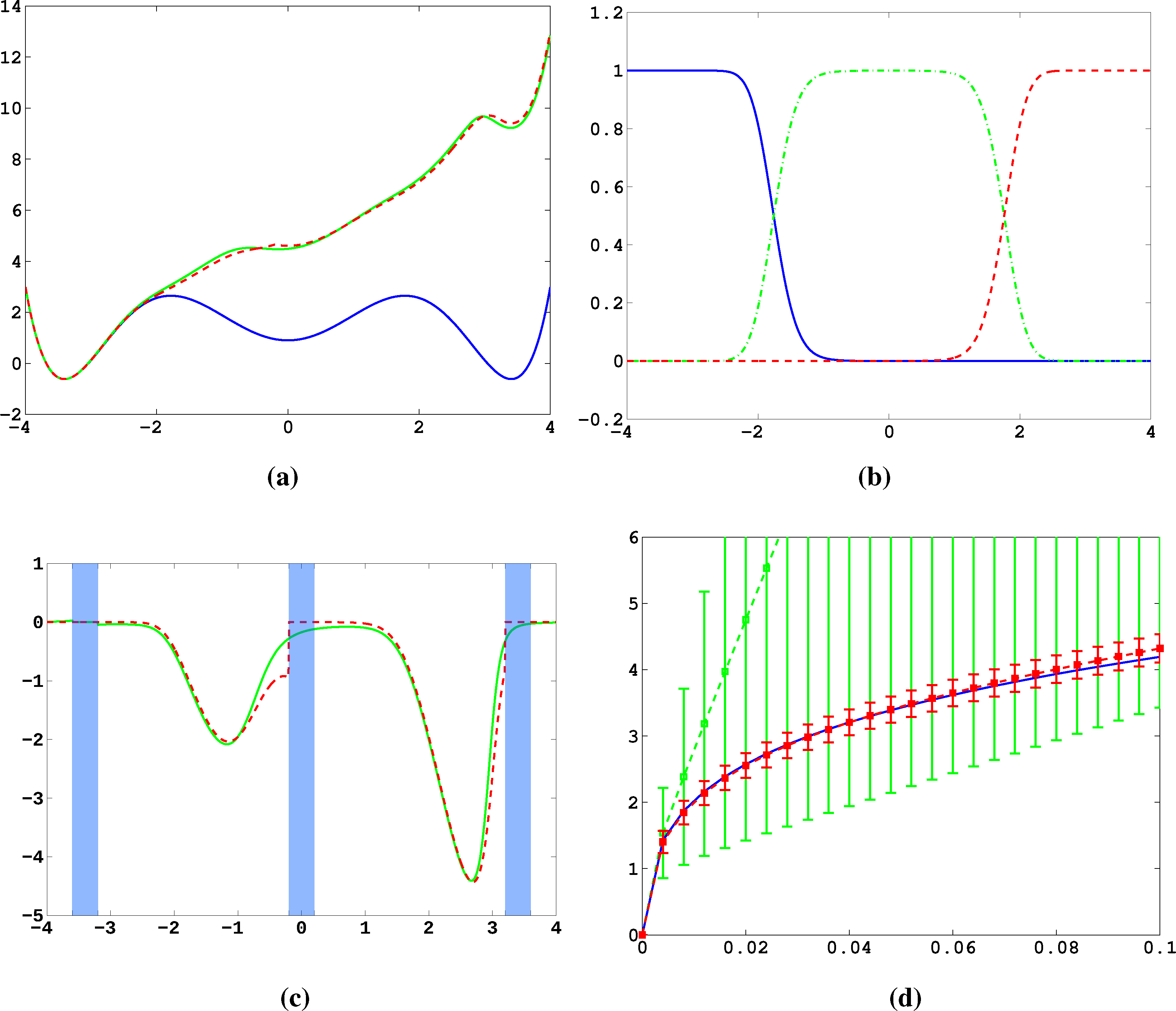
Firstly, we study diffusion in the triple well potential, which is presented in Figure 2. This potential has three minima at approximately x0/1 = ±3.4 and x2 = 0. We choose the three core sets Ci = [xi − δ, xi + δ] around the minima with δ = 0.2. Take τ to be the first hitting time of C0. We are interested in the moment generating function ϕ(x) = 𝔼[e−∊−1στ] of passages into C0 and the cumulant generating function W = ∊log ϕ. This is of the form Equation (32) for A = Ci and f = σ, a constant function.
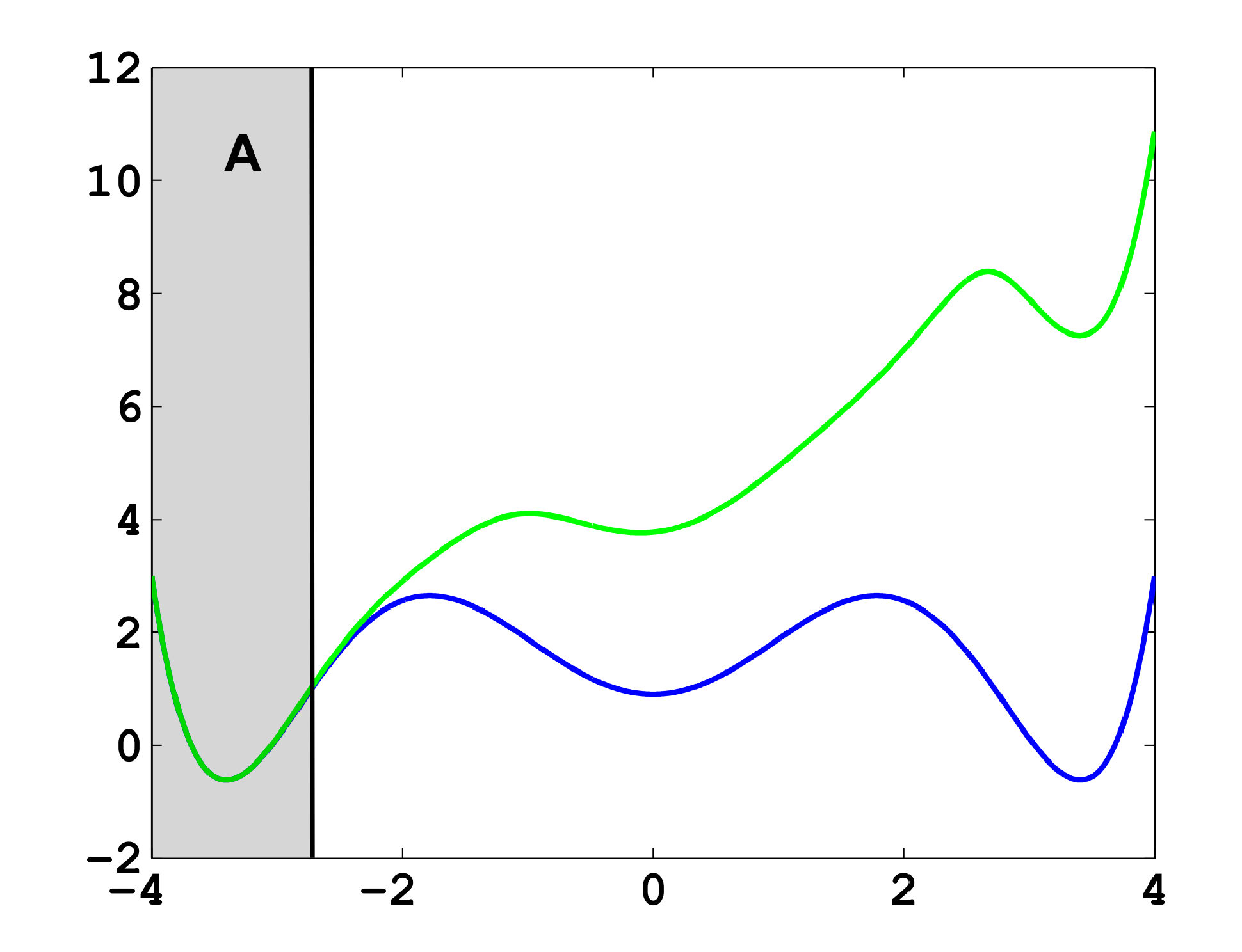
In Figure 11a, the potential, V, and effective potential, U, are shown for β = 2 and σ = 0.08 (solid lines), cf. Equation (30). One can observe that the optimal control effectively lifts the second and third well up, which means that the optimal control will drive the system into C0 very quickly. The reference computations here have been carried out using a full partition FEM (finite element method) discretization of Equation (31) with a lattice spacing of h = 0.01. Now, we study the MJP approximation constructed via the committor functions shown in Figure 11b. These span a three-dimensional subspace, but due to the boundary conditions, the subspace, D, of the method is actually two-dimensional. The dashed line in Figure 11a gives the approximation to U calculated by solving Equation (38). We can observe extremely good approximation quality, even in the transition region. In Figure 11c, the approximation to the optimal control, α*(x) (solid line), and its approximation α̂* = −▿Ŵ (dashed line) are shown. The core sets are shown in blue. We can observe jumps in α̂* at the left boundaries of the core sets. This is to be expected and comes from the fact that the committor functions are not smooth at the boundaries of the core sets, but only continuous. Therefore, the approximation to U is continuous, but the approximation to α* is not.
Next, we construct a core MSM to sample the matrices, K and F. One hundred trajectories of length T = 20, 000 were used to build the MSM. In Figure 11d, W and its estimate using the core MSM are shown for ∊ = 0.5 and different values of σ. Each of the 100 trajectories has seen about four transitions. For comparison, a direct sampling estimate of W using the same data is shown (green). The direct sampling estimate suffers from a large bias and variance and is practically useless. In contrast, the MSM estimator for W performs well for all considered values of σ, and always, its variance is significantly small. The constant, C, which ensures ϕ̂ > 0 when σ ≤ C, is approximately 0.2 in this case. This seems restrictive, but still allows one to capture all interesting information about ϕ and W.
10.2. Alanine Dipeptide
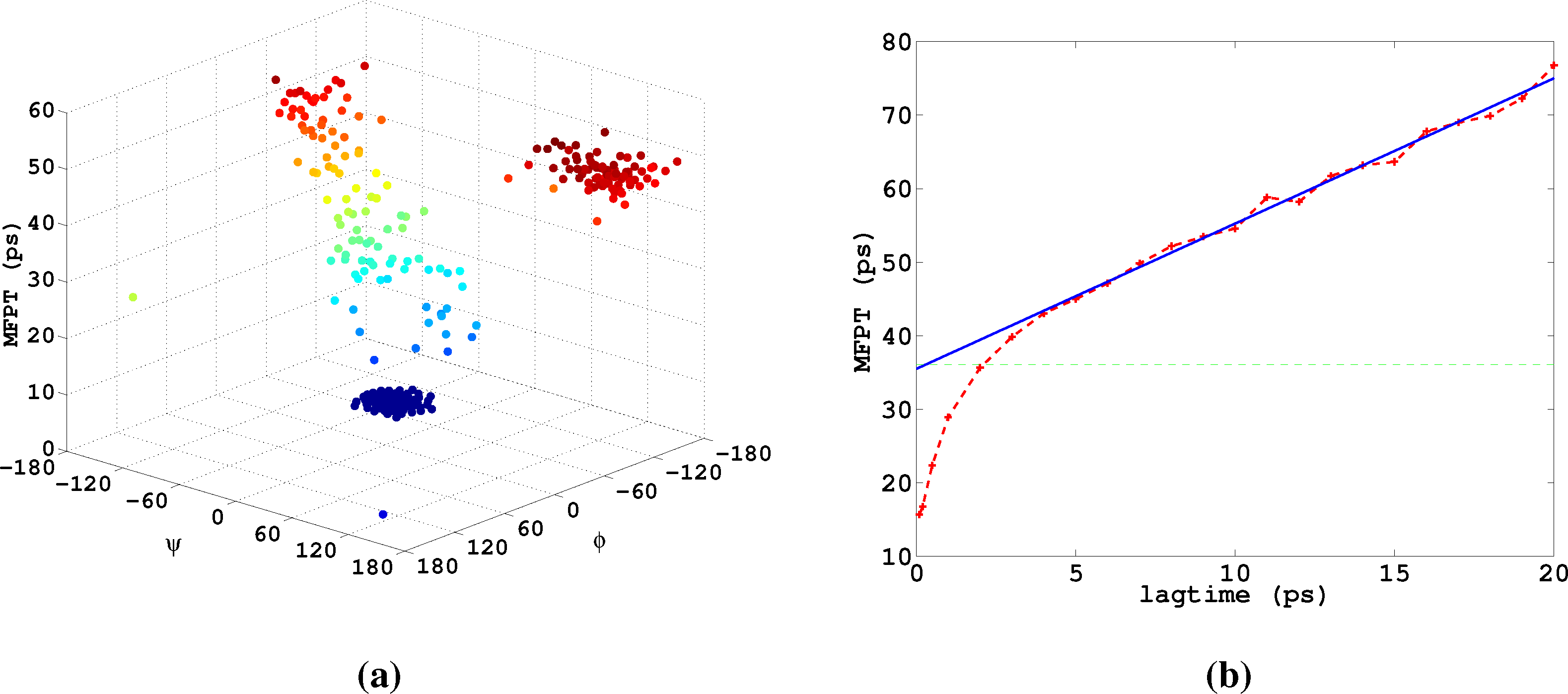
Lastly, we study α-β-transitions in alanine dipeptide, a well-studied test system for molecular dynamics applications. We use a 1μs long trajectory simulated with the CHARMM (Chemistry at HARvard Molecular Mechanics) 27 force field. The conformational dynamics is monitored as usual via the backbone dihedral angles, ϕ and ψ. The data was first presented in [27]. We construct a full partition MSM with 250 clusters using k-means clustering. We are interested in the MFPT (mean first passage time) t̂(i) = 𝔼i[τα], where τα is the first hitting time of the α conformation, which we define as a circle with radius r = 45 around (ϕα,ψα) = (−80, −60). The MFPT vector, t̂, solves the boundary value problem
In [14], it is demonstrated how to use the method presented herein for maximizing the population of the α-conformation of alanine dipeptide based on the MSM used here.
11. Conclusions
In this article, we have discussed an approach to overcome direct sampling issues of rare events in molecular dynamics based on spatial discretization of the molecular state space. The strategy is to define a discretization by subsets of state space, such that the sampling effort with respect to transitions between the sets is much lower than the direct estimation of the rare events under consideration. That is, without having to simulate rare events, we construct a so-called Markov State Model, a Markov chain approximation to the original dynamics. Since the state space of the MSM is finite, we can then calculate the properties of interest by simply solving linear systems of equations. Of course, it is crucial that these properties of the MSM can be related to the rare event properties of the original process that we have not been able to sample directly.
This is why we have analyzed the approximation quality of MSMs in the first part of the article. We have used the interpretation of MSMs as projections of the transfer operator to: (1) derive conditions that guarantee an accurate reproduction of the dynamics; and (2) show how to construct models based on a core set discretization by leaving the state space partly undiscretized.
In the second part of the article, we have used the concept of MSM discretization to solve MD optimal control problems in which one computes the optimal external force that drives the molecular system to show an optimized behavior (maximal possible population in a conformation; minimal mean first passage time to a certain conformation) under certain constraints. We have demonstrated that the spatial discretization underlying an MSM turns the high-dimensional continuous optimal control problem into a rather low-dimensional discrete optimal control problem of the same form that can be solved efficiently. This result allows two different types of applications: (1) if one can construct an MSM for a molecular system in equilibrium, then one can use it to compute optimal controls that extremize a given costs criterion; (2) if an MSM can be computed based on transition probabilities between neighboring core sets alone, then the rare event statistics for transitions between strongly separated metastable states of the system can be computed from an associated optimal control problem that can be solved after discretization using the pre-computed MSM.
Acknowledgments
The authors have been supported by the DFG Research Center MATHEON.
Conflicts of Interest
The authors declare no conflict of interest.
References
- Hartmann, C.; Banisch, R.; Sarich, M.; Badowski, T.; Schütte, C. Characterization of rare events in molecular dynamics. Entropy 2014, 16, 350–376. [Google Scholar]
- Metzner, P.; Schütte, C.; Vanden-Eijnden, E. Transition path theory for markov jump processes. Multiscale Model. Simul 2009, 7, 1192–1219. [Google Scholar]
- Pan, A.C.; Roux, B. Building Markov state models along pathways to determine free energies and rates of transitions. J. Chem. Phys 2008, 129, 064107. [Google Scholar]
- Noé, F.; Schütte, C.; vanden-Eijnden, E.; Reich, L.; Weikl, T. Constructing the full ensemble of folding pathways from short off-equilibrium trajectories. Proc. Natl. Acad. Sci. USA 2009, 106, 19011–19016. [Google Scholar]
- Schütte, C. Conformational Dynamics: Modelling, Theory, Algorithm, and Applications to Biomolecules. Habilitation Thesis, Fachbereich Mathematik und Informatik, Freie Universität Berlin, Berlin, Germany,. 1998. [Google Scholar]
- Schütte, C.; Fischer, A.; Huisinga, W.; Deuflhard, P. A direct approach to conformational dynamics based on hybrid monte Carlo. J. Comput. Phys 1999, 151, 146–168. [Google Scholar]
- Prinz, J.H.; Wu, H.; Sarich, M.; Keller, B.; Fischbach, M.; Held, M.; Chodera, J.D.; Schütte, C.; Noé, F. Markov models of molecular kinetics: Generation and validation. J. Chem. Phys 2011, 134, 174105. [Google Scholar]
- Noé, F.; Horenko, I.; Schütte, C.; Smith, J.C.. Hierarchical analysis of conformational dynamics in biomolecules: Transition networks of metastable states. J. Chem. Phys 2007, 126, 155102. [Google Scholar]
- Chodera, J.D.; Dill, K.A.; Singhal, N.; Pande, V.S.; Swope, W.C.; Pitera, J.W. Automatic discovery of metastable states for the construction of Markov models of macromolecular conformational dynamics. J. Chem. Phys 2007, 126, 155101. [Google Scholar]
- Buchete, N.V.; Hummer, G. Coarse master equations for peptide folding dynamics. J. Phys. Chem. B 2008, 112, 6057–6069. [Google Scholar]
- Prinz, J.H.; Keller, B.; Noé, F. Probing molecular kinetics with Markov models: Metastable states, transition pathways and spectroscopic observables. Phys. Chem. Chem. Phys 2011, 13, 16912–16927. [Google Scholar]
- Keller, B.; Prinz, J.H.; Noé, F. Markov models and dynamical fingerprints: Unraveling the complexity of molecular kinetics. Chem. Phys 2011. in press.. [Google Scholar]
- Bowman, G.; Volez, V.; Pande, V.S.. Taming the complexity of protein folding. Curr. Opin. Struct. Biol 2011, 21, 4–11. [Google Scholar]
- Schütte, C.; Winkelmann, S.; Hartmann, C. Optimal control of molecular dynamics using Markov state models. Math. Program. Ser. B 2012, 134, 259–282. [Google Scholar]
- Hartmann, C.; Schütte, C. Efficient rare event simulation by optimal nonequilibrium forcing. J. Stat. Mech. Theor. Exp 2012. [Google Scholar] [CrossRef]
- Jäger, M.; Zhang, Y.; Bieschke, J.; Nguyen, H.; Dendle, M.; Bowman, M.E.; Noel, J.P.; Gruebele, M.; Kelly, J.W. Structure-function-folding relationship in a WW domain. Proc. Natl. Acad. Sci. USA 2006, 103, 10648–10653. [Google Scholar]
- Kobitski, A.Y.; Nierth, A.; Helm, M.; Jäschke, A.; Nienhaus, G.U.. Mg2+ dependent folding of a Diels-Alderase ribozyme probed by single-molecule FRET analysis. Nucleic Acids Res 2007, 35, 2047–2059. [Google Scholar]
- Fischer, S.; Windshuegel, B.; Horak, D.; Holmes, K.C.; Smith, J.C.. Structural mechanism of the recovery stroke in the Myosin molecular motor. Proc. Natl. Acad. Sci. USA 2005, 102, 6873–6878. [Google Scholar]
- Noé, F.; Krachtus, D.; Smith, J.C.; Fischer, S. Transition networks for the comprehensive characterization of complex conformational change in proteins. J. Chem. Theory Comput 2006, 2, 840–857. [Google Scholar]
- Ostermann, A.; Waschipky, R.; Parak, F.G.; Nienhaus, U.G.. Ligand binding and conformational motions in myoglobin. Nature 2000, 404, 205–208. [Google Scholar]
- Huisinga, W. Metastability of Markovian Systems a Transfer Operator Based Approach in Application to Molecular Dynamics. Ph.D Thesis, Fachbereich Mathematik und Informatik, Freie Universität Berlin, Berlin, Germany,. 2001. [Google Scholar]
- Bovier, A.; Eckhoff, M.; Gayrard, V.; Klein, M. Metastability in reversible diffusion processes. I. Sharp asymptotics for capacities and exit times. J. Eur. Math. Soc 2004, 6, 399–424. [Google Scholar]
- Voronoi, M.G. Nouvelles applications des parametres continus a la theorie des formes quadratiques. J. Reine Angew. Math 1908, 134, 198–287. [Google Scholar]
- Sarich, M.; Noé, F.; Schütte, C. On the approximation quality of markov state models. Multiscale Model. Simul 2010, 8, 1154–1177. [Google Scholar]
- Sarich, M. Projected Transfer Operators. Ph.D. Thesis, Freie Universität Berlin, Berlin, Germany,. 2011. [Google Scholar]
- Sarich, M.; Schütte, C. Approximating selected non-dominant timescales by Markov state models. Commun. Math. Sci 2012, 10, 1001–1013. [Google Scholar]
- Schütte, C.; Noé, F.; Lu, J.; Sarich, M.; Vanden-Eijnden, E. Markov state models based on milestoning. J. Chem. Phys 2011, 134, 204105. [Google Scholar]
- Faradjian, A.K.; Elber, R. Computing time scales from reaction coordinates by milestoning. J. Chem. Phys 2004, 120, 10880–10889. [Google Scholar]
- Roeblitz, S. Statistical Error Estimation and Grid-free Hierarchical Refinement in Conformation Dynamics. Ph.D. Thesis, Freie Universität Berlin, Berlin, Germany,. 2008. [Google Scholar]
- Djurdjevac, N.; Sarich, M.; Schütte, C. On Markov State Models for Metastable Processes. In Proceeding of the ICM 2010 as Invited Lecture, Hyderabad, India, 19–27 August 2010; Available online: http://www.biocomputing-berlin.de/biocomputing/en/?cmd=publication (accessed on 29 November 2010).
- Horenko, I.; Dittmer, E.; Lankas, F.; Maddocks, J.; Metzner, P.; Schütte, C. Macroscopic dynamics of complex metastable systems: Theory, algorithms, and application to B-DNA. J. Appl. Dyn. Syst 2008, 7, 532–560. [Google Scholar]
- Weber, M.; Bujotzek, A.; Haag, R. Quantifying the rebinding effect in multivalent chemical ligand-receptor systems. J. Chem. Phys 2012, 137, 054111. [Google Scholar]
- Bowmana, G.R.; Huangb, X.; Pande, V.S.. Using generalized ensemble simulations and Markov state models to identify conformational states. Methods 2009, 49, 197–201. [Google Scholar]
- Schütte, C.; Sarich, M. Metastability and Markov State Models in Molecular Dynamics. Modeling, Analysis, Algorithmic Approaches (Courant Lecture Notes No. 24); AMS: Providence, RI, USA, 2013. [Google Scholar]
- Weber, M.; Fackeldey, K. Computing the minimal rebinding effect included in a given kinetics. Multiscale Model. Simul 2013. Available onlin: http://www.zib.de/en/numerik/publications.html (accessed on 1 December 2013). [Google Scholar]
- Fleming, W.; Soner, H. Controlled Markov Processes and Viscosity Solutions, 2nd ed.; Springer: New York, NY, USA, 2005. [Google Scholar]
- Oksendal, B. Stochastic Differential Equations; Springer: Heidelberg, Germany, 2003. [Google Scholar]
- Pra, P.; Meneghini, L.; Runggaldier, W. Connections between stochastic control and dynamic games. Math. Control Signals Syst 1996, 9, 303–326. [Google Scholar]
- Kushner, H.; Dupuis, P. Numerical Methods for Stochastic Control Problems in Continuous Time; Springer Verlag: New York, NY, USA, 1992. [Google Scholar]
- Braess, D. Finite Elements: Theory, Fast Solvers and Applications in Solid Mechanics; Cambridge University Press: Camebridge, UK, 2007. [Google Scholar]
- Banisch, R.; Hartmann, C. A meshfree discretization for optimal control problems. SIAM J. Control Optim 2013. submitted.. [Google Scholar]
- Sheu, S. Stochastic control and exit probabilities of jump processes. SIAM J. Control Optim 1985, 23, 306–328. [Google Scholar]
- Latorre, J.; Metzner, P.; Hartmann, C.; Schütte, C. A Structure-preserving numerical discretization of reversible diffusions. Commun. Math. Sci 2011, 9, 1051–1072. [Google Scholar]
- Chodera, J.D.; Elms, P.J.; Swope, W.C.; Prinz, J.H.; Marqusee, S.; Bustamante, C.; Noé, F.; Pande, V.S.. A robust approach to estimating rates from time-correlation Functions. 2011. arXiv:1108.2304. [Google Scholar]
- Vanden-Eijnden, E. Transition path theory. In Computer Simulations in Condensed Matter Systems: From Materials to Chemical Biology Volume 1; Ferrario, M., Ciccotti, G., Binder, K., Eds.; Springer: Berlin/Heidelberg, Gemary, 2006; Volume 703, pp. 353–493. [Google Scholar]


| T1 | T2 | |
|---|---|---|
| Original | 103.7608 | 11.9566 |
| Full partition 3 sets | 80.6548 | 9.8784 |
| T1 | T2 | |
|---|---|---|
| Original | 103.7608 | 11.9566 |
| 3 core sets | 100.8066 | 11.9145 |
| Full partition 3 sets | 80.6548 | 9.8784 |
© 2014 by the authors; licensee MDPI, Basel, Switzerland This article is an open access article distributed under the terms and conditions of the Creative Commons Attribution license (http://creativecommons.org/licenses/by/3.0/).
Share and Cite
Sarich, M.; Banisch, R.; Hartmann, C.; Schütte, C. Markov State Models for Rare Events in Molecular Dynamics. Entropy 2014, 16, 258-286. https://doi.org/10.3390/e16010258
Sarich M, Banisch R, Hartmann C, Schütte C. Markov State Models for Rare Events in Molecular Dynamics. Entropy. 2014; 16(1):258-286. https://doi.org/10.3390/e16010258
Chicago/Turabian StyleSarich, Marco, Ralf Banisch, Carsten Hartmann, and Christof Schütte. 2014. "Markov State Models for Rare Events in Molecular Dynamics" Entropy 16, no. 1: 258-286. https://doi.org/10.3390/e16010258