Blind Demodulation of Chaotic Direct Sequence Spread Spectrum Signals Based on Particle Filters

Abstract

Applying the particle filter (PF) technique, this paper proposes a PF-based algorithm to blindly demodulate the chaotic direct sequence spread spectrum (CDS-SS) signals under the colored or non-Gaussian noises condition. To implement this algorithm, the PFs are modified by (i) the colored or non-Gaussian noises are formulated by autoregressive moving average (ARMA) models, and then the parameters that model the noises are included in the state vector; (ii) the range-differentiating factor is imported into the intruder’s chaotic system equation. Since the range-differentiating factor is able to make the inevitable chaos fitting error advantageous based on the chaos fitting method, thus the CDS-SS signals can be demodulated according to the range of the estimated message. Simulations show that the proposed PF-based algorithm can obtain a good bit-error rate performance when extracting the original binary message from the CDS-SS signals without any knowledge of the transmitter’s chaotic map, or initial value, even when colored or non-Gaussian noises exist.

1. Introduction

Chaotic signals exhibit several special characteristics such as extraordinary sensitivity to initial conditions, aperiodicity, broad Fourier transform spectra and high security, which coincide with the requirements for signals used in secure communication systems [1,2,3,4]. In secure communication, chaotic signals make the received signals seem like noises, thereby hiding the transmitted messages efficiently and securely. So far, a large number of chaotic secure communication schemes have been advanced in the last decades, including chaotic masking [1], chaotic shift keying [2], chaotic modulation [3], and chaotic direct sequence spread spectrum (CDS-SS) [4].

CDS-SS, where a binary message is multiplied by the chaotic carrier and encrypted into a CDS-SS signal, has been extensively studied as an approach of chaotic secure communication owing to its relatively good security [5,6,7]. Hwang [6] demonstrated that CDS-SS has the merit of physical-layer security, and Yu [7] showed that CDS-SS has a low probability of interception. Therefore, the research on the blind demodulation of CDS-SS signals is considered to have great prospects for communication management and military reconnaissance, also it can guide the further improvement of CDS-SS schemes’ security. Viewed from the principle of demodulation in the chaotic communication field, most demodulation methods are based on two major characteristics of chaotic secure communications. The first characteristic is that there are two chaotic attractors, where a binary message is encoded into two different chaotic attractors. The second one is that the relation of the message and the chaotic carrier is completely additive. However, CDS-SS has neither of the two characteristics [6,7]. In CDS-SS, the relation between the message and the chaotic carrier is multiplicative and there is only one chaotic attractor, so existent demodulation methods are inapplicable to CDS-SS. So far, many works [8,9,10,11,12,13,14] break chaotic secure communications with the requirement that the structure of the chaotic map is given. Sameh et al. [8] develop a particle filter (PF) algorithm to solve the problem of chaotic state and unknown additive input estimation even if Gaussian or non-Gaussian noises that are known exist in the chaotic maps. Some approaches [9,10] estimate simultaneously the state of the system and the unknown inputs using a generalized state space observer. Seongkeun et al. [11] developed a Maximun A Posteriori-particle filter (MAP-PF) to estimate not only the chaotic state, but also the secure message which is added directly to the chaotic carrier. Xu et al. [12] proposed an adaptive bidirectionally coupled synchronization method to estimate the chaotic states with unknown parameters. Several researchers [13,14] have developed adaptive control based approaches to estimate the states of chaotic systems with uncertain parameters and uncertain disturbances. However, when the structure of the chaotic map (i.e., the transmitter’s structure) is unknown for the non-cooperative communication condition, the methods mentioned above will be disabled. Hu and Guo [15] proposed a modified unscented Kalman filter to blindly demodulate the CDS-SS signals relying on the white Gaussian approximation which is a very stringent assumption in practical communication systems. A nonlinear Resilient back PROpagation (RPROP) neural network was proposed to estimate the chaotic sequences without knowing the transmitter’s structure under the additive white Gaussian noise (AWGN) condition [16], but the RPROP neural network method requires a training sequence that passes through the CDS-SS communication system to identify the unknown transmitter’s system, which can be hardly implemented in practice. In short, most works [5,8,9,10,11,12,13,14,15,16,17,18,19,20,21] have considered demodulating the chaotic secure communication systems with the assumptions that: (i) the transmitter’s structure is known, and even that the parameters are given; or (ii) chaotic maps and their time series are only affected by white noise, in particular Gaussian noise.

In this study, the particle filtering technique is employed to solve the problems mentioned above. The particle filter (PF) is the state-of-the-art solution to nonlinear and non-Gaussian problem, following the Bayesian filtering framework, which uses a sequential Monter Carlo method to approximate the optimal filtering by representing the probability density function with a swarm of particles [22,23,24]. Due to this sample-based representation, particle filters are able to represent a wide range of probability densities, allowing online, real-time estimation of nonlinear, colored or non-Gaussian dynamic systems. Li and Feng [25] prove that the PF has better performance in convergence rate and estimation accuracy than the extended Kalman filter (EKF) and unscented Kalman filter (UKF).

In this paper, a novel PF-based algorithm is proposed to blindly demodulate the CDS-SS communication system without any knowledge of the transmitter’s chaotic map, parameters, or initial value, and even under colored or non-Gaussian noise conditions. To begin with, the formulation of this problem is introduced. Then, autoregressive moving average (ARMA) models are utilized to describe the colored noises, so that the demodulation could be formulated as a mixed parameter and state estimation problem. Accordingly, the message signal can be estimated by using two alternate PFs, and the state variable of one PF is the chaotic state, and the other one is the message signal. Finally, the proposed algorithm is implemented to blindly demodulate the CDS-SS signals.

2. Problem Formulation

Consider a CDS-SS communication system, in which the transmitter’s chaotic system is described by:

$$x_{k+1}=f(x_k)$$

(1)

The chaotic spreading sequence $\left\{x_k\right\}$ is supposed to be a simple one that is generated by one chaotic map that is doubly symmetrical, i.e., the range of its values and its probability distribution are both symmetrical [5,19]. Each original binary message $b_n\in \left\{-1,1\right\}$ is associated with a string of N elements $x_k(k=(n-1)N+1,\cdots ,nN)$, where N is the spreading factor. Namely, $b_n$ is encoded as the string:

$$s_k=b_n{x}_k\text{，}k=(n-1)N+1,\cdots ,nN\text{，}n=1,2,\cdots$$

(2)

Let $b_n=b_k,k=(n-1)N+1,\cdots ,nN$, then Equation (2) is rewritten as $s_k=b_k{x}_k$. Since the transmitter’s chaotic map is unknown, the intruder uses another chaotic map $g(\cdot )$ instead of $f(\cdot )$, and its chaotic system equation is given by:

$${\widehat{x}}_{k+1}=g({\widehat{x}}_k)$$

(3)

Because the transmitted CDS-SS signal is $s_{k+1}=b_{k+1}f(x_k)$, the CDS-SS signal estimated by the intruder could be ${\widehat{s}}_{k+1}={\widehat{b}}_{k+1}g({\widehat{x}}_k)$, where $\widehat{b}$ and $\widehat{x}$ are the estimation of b and x, respectively. Considering the model error or noise, the following system and measurement equations [15] can be obtained:

$$\{\begin{array}{l}{\widehat{x}}_{k+1}=g({\widehat{x}}_k)+w_k^{(1)}\\ z_{k+1}=\mathrm{sgn}({\widehat{b}}_{k+1}){\widehat{x}}_{k+1}+v_{k+1}^{(1)}\end{array}$$

(4)

where $z_{k+1}$ is the observation, $v_{k+1}^{(1)}$ is the measurement noise with zero-mean and arbitrary distribution, $w_k^{(1)}$ is the colored or non-Gaussian process noise that drives the dynamic systems through the nonlinear state transition function. On the other hand, since the message $b_k$ in CDS-SS varies more slowly than the chaotic sequence $\left\{x_k\right\}$, ${\widehat{b}}_{k+1}={\widehat{b}}_k$ approximately. Thus, the system and measurement equations can also be written as:

$$\{\begin{array}{l}{\widehat{b}}_{k+1}={\widehat{b}}_k+w_k^{(2)}\\ z_{k+1}={\widehat{b}}_{k+1}g({\widehat{x}}_k)+v_{k+1}^{(2)}\end{array}$$

(5)

where $\mathrm{sgn}({\widehat{b}}_{k+1})=1$ (if ${\widehat{b}}_{k+1}>0$) or $\mathrm{sgn}({\widehat{b}}_{k+1})=-1$ (if ${\widehat{b}}_{k+1}<0$), $v_{k+1}^{(2)}$ is the measurement noise with zero-mean and arbitrary distribution, $w_k^{(2)}$ is the colored or non-Gaussian process noise that drive the dynamic systems through the nonlinear state transition function.

The colored noises $w_k^{(1)}$ and $w_k^{(2)}$ can be formulated by ARMA models [26] as:

$$w_k^{(1)}+c_1^{(1)}{w}_{k-1}^{(1)}+c_2^{(1)}{w}_{k-2}^{(1)}+\cdot \cdot \cdot +c_{p_1}^{(1)}{w}_{k-p_1}^{(1)}=n_k^{(1)}+d_1^{(1)}{n}_{k-1}^{(1)}+d_2^{(1)}{n}_{k-2}^{(1)}+\cdot \cdot \cdot +d_{q_1}^{(1)}{n}_{k-q_1}^{(1)}$$

(6)

$$w_k^{(2)}+c_1^{(2)}{w}_{k-1}^{(2)}+c_2^{(2)}{w}_{k-2}^{(2)}+\cdot \cdot \cdot +c_{p_2}^{(2)}{w}_{k-p_2}^{(2)}=n_k^{(2)}+d_1^{(2)}{n}_{k-1}^{(2)}+d_2^{(2)}{n}_{k-2}^{(2)}+\cdot \cdot \cdot +d_{q_2}^{(2)}{n}_{k-q_2}^{(2)}$$

(7)

Let:

$$C^{(i)}=\left[\begin{array}{cccc}{c}_1^{(i)}& c_2^{(i)}& \cdot \cdot \cdot & c_{p_i}^{(i)}\end{array}\right]\text{for }i=1,2.$$

(8)

$$D^{(i)}=\left[\begin{array}{cccc}{d}_1^{(i)}& d_2^{(i)}& \cdot \cdot \cdot & d_{q_i}^{(i)}\end{array}\right]\text{for }i=1,2.$$

(9)

$$T^{(i)}=\left[\begin{array}{cc}-C^{(i)}& D^{(i)}\end{array}\right]\text{for }i=1,2.$$

(10)

Furthermore, let:

$${\tilde{x}}_k={\left[\begin{array}{cccccccc}{w}_{k-1}^{(1)}& w_{k-2}^{(1)}& \cdot \cdot \cdot & w_{k-p_1}^{(1)}& n_{k-1}^{(1)}& n_{k-2}^{(1)}& \cdot \cdot \cdot & n_{k-q_1}^{(1)}\end{array}\right]}^T$$

(11)

$${\tilde{b}}_k={\left[\begin{array}{cccccccc}{w}_{k-1}^{(2)}& w_{k-2}^{(2)}& \cdot \cdot \cdot & w_{k-p_2}^{(2)}& n_{k-1}^{(2)}& n_{k-2}^{(2)}& \cdot \cdot \cdot & n_{k-q_2}^{(2)}\end{array}\right]}^T$$

(12)

where ${\tilde{x}}_k$ satisfies:

$$\begin{array}{c}{\tilde{x}}_{k+1}=\left[\begin{array}{lllllllll}-c_1^{(1)}& -c_2^{(1)}& \cdots & \cdots & -c_{p_1}^{(1)}& d_1^{(1)}& d_2^{(1)}& \cdots & d_{q_1}^{(1)}\\ 1& & & & 0& & & & \\ & 1& & & ⋮& & & & \\ & & \ddots & & ⋮& & & & \\ & & & 1& 0& & & & \\ & & & & & 0& 0& \cdots & 0\\ & & & & & 1& & & ⋮\\ & & & & & & \ddots & & ⋮\\ & & & & & & & 1& 0\end{array}\right]{\tilde{x}}_k+\left[\begin{array}{c}1\\ 0\\ ⋮\\ 0\\ -\\ 1\\ 0\\ ⋮\\ 0\end{array}\right]n_k^{(1)}\\ ={\tilde{A}}_1{\tilde{x}}_k+{\tilde{B}}_1{n}_k^{(1)}\end{array}$$

(13)

and ${\tilde{b}}_k$ satisfies:

$$\begin{array}{c}{\tilde{b}}_{k+1}=\left[\begin{array}{lllllllll}-c_1^{(2)}& -c_2^{(2)}& \cdots & \cdots & -c_{p_2}^{(2)}& d_1^{(2)}& d_2^{(2)}& \cdots & d_{q_2}^{(2)}\\ 1& & & & 0& & & & \\ & 1& & & ⋮& & & & \\ & & \ddots & & ⋮& & & & \\ & & & 1& 0& & & & \\ & & & & & 0& 0& \cdots & 0\\ & & & & & 1& & & ⋮\\ & & & & & & \ddots & & ⋮\\ & & & & & & & 1& 0\end{array}\right]{\tilde{b}}_k+\left[\begin{array}{c}1\\ 0\\ ⋮\\ 0\\ -\\ 1\\ 0\\ ⋮\\ 0\end{array}\right]n_k^{(2)}\\ ={\tilde{A}}_2{\tilde{b}}_k+{\tilde{B}}_2{n}_k^{(2)}\end{array}$$

(14)

Then, the state vectors are augmented as ${\overline{x}}_k={\left[\begin{array}{cc}{\widehat{x}}_k& {\tilde{x}}_k^T\end{array}\right]}^T$ and ${\overline{b}}_k={\left[\begin{array}{cc}{\widehat{b}}_k& {\tilde{b}}_k^T\end{array}\right]}^T$. Therefore, the augmented state-space models corresponding to Equations (4) and (5) can be rewritten as:

$$\{\begin{array}{c}\begin{array}{l}{\overline{x}}_{k+1}=\left[\begin{array}{c}g({\widehat{x}}_k)\\ 0\end{array}\right]+\left[\begin{array}{c}{T}^{(1)}\\ {\tilde{A}}_1\end{array}\right]{\tilde{x}}_k+\left[\begin{array}{c}1\\ {\tilde{B}}_1\end{array}\right]n_k^{(1)}\\ =\left[\begin{array}{c}g({\widehat{x}}_k)\\ 0\end{array}\right]+{\overline{A}}_1{\tilde{x}}_k+{\overline{B}}_1{n}_k^{(1)}\end{array}\\ z_{k+1}=\mathrm{sgn}({\widehat{b}}_{k+1}){\widehat{x}}_{k+1}+v_{k+1}^{(1)}\end{array}$$

(15)

$$\{\begin{array}{c}\begin{array}{l}{\overline{b}}_{k+1}=\left[\begin{array}{c}{\widehat{b}}_k\\ 0\end{array}\right]+\left[\begin{array}{c}{T}^{(2)}\\ {\tilde{A}}_2\end{array}\right]{\tilde{b}}_k+\left[\begin{array}{c}1\\ {\tilde{B}}_2\end{array}\right]n_k^{(2)}\\ =\left[\begin{array}{c}{\widehat{b}}_k\\ 0\end{array}\right]+{\overline{A}}_2{\tilde{b}}_k+{\overline{B}}_2{n}_k^{(2)}\end{array}\\ z_{k+1}={\widehat{b}}_{k+1}g({\widehat{x}}_k)+v_{k+1}^{(2)}\end{array}$$

(16)

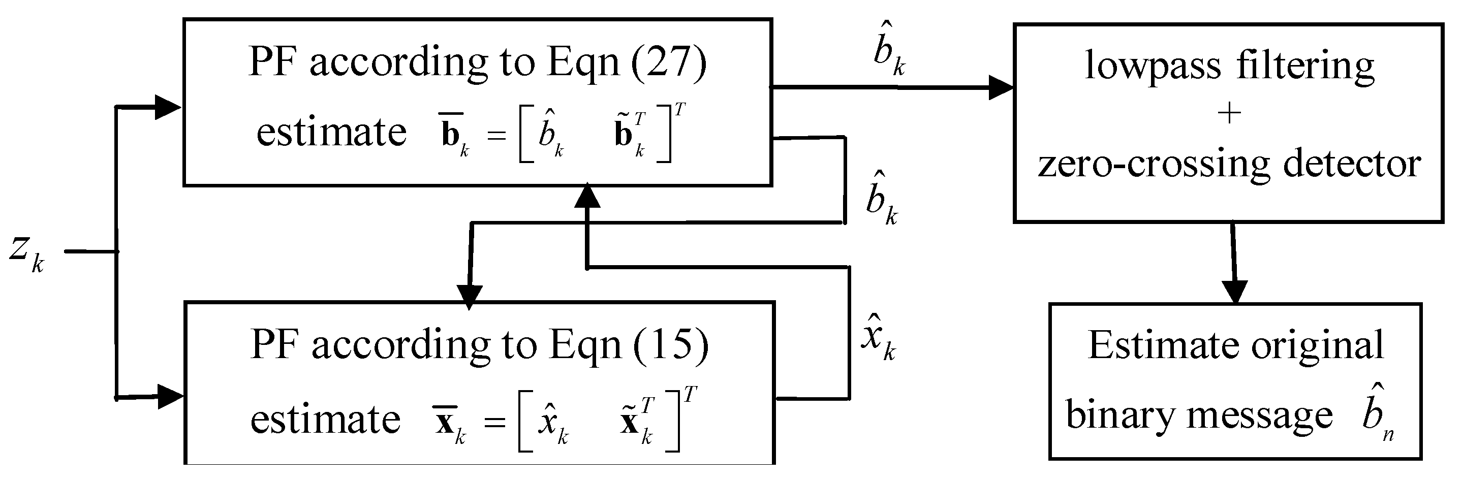
3. Blind Demodulation of CDS-SS Signals Based on Particle Filters

3.1. Particle Filter

To begin with, a brief review of the PF is described first [22,23,24]. Let us consider a dynamic system represented by:

$${\mathbf{x}}_{k+1}=f({\mathbf{x}}_k)+{\mathbf{w}}_k$$

(17)

$${\mathbf{z}}_{k+1}=h(x_{k+1})+{\mathbf{v}}_{k+1}$$

(18)

where $x_k$ is the state vector, $z_k$ is the measurement vector, $f(\cdot )$ and $h(\cdot )$ are system and measurement equations, respectively, and $w_k$ and $v_k$ are process and measurement noises, respectively. Unlike the conventional analytical approximation methods, PFs are commonly used for the approximation of intractable integrals and rely on the ability to draw random samples (or particles) from a probability distribution. The main idea is to represent the posterior probability density function of the target state by a set of random particles ${\left\{x_k^j\right\}}_{j=1}^M$ with their associated weights ${\left\{{\lambda }_k^j\right\}}_{j=1}^M$, where k is the time step, j is the particle index, and M is the particle number, i.e.:

$$p(x_k|z_{1:k})=\frac{1}{{\overline{\lambda }}_k}{\displaystyle {\sum }_{j=1}^M{\lambda }_k^j\delta (x_k-x_k^j)}$$

(19)

operations where ${\overline{\lambda }}_k={\displaystyle {\sum }_{j=1}^M{\lambda }_k^j}$ , $\delta (\cdot )$ is the Dirac delta function, $z_{1:k}=\left\{z_1,z_2,\dots ,z_k\right\}$ is the set of accumulated measurements up to the kth time step. Then, one can compute an optimal estimate based on these particles and weights. In the processing of PFs, generally there are six important steps:

(i) Initialization

Begin by generating M particles ${\left\{{\mathbf{x}}_0^j\right\}}_{j=1}^M$ from $p({\mathbf{x}}_0)$ which is the initial probability for the state;

(ii) Prediction/sampling

Sample new particles $x_{k+1}^j~\pi (x_{k+1}|x_k^j,z_{1:k+1})$ $j=1,\mathrm{...},M$, where $\pi (x_{k+1}|x_n^j,z_{1:k+1})$ is the proposed distribution. The most popular choice of the proposed distribution is the prior transition $\pi (x_{k+1}|x_k^j,z_{1:k+1})=p(x_{k+1}|x_k^j)$ due to its simplicity;

(iii) Measurement update

For $j=1,2,\cdot \cdot \cdot ,M$, update the weights by the likelihood:

$$\begin{array}{l}{\lambda }_{k+1}^j={\lambda }_k^{j}p(z_{k+1}|x_{k+1}^j)\\ \text{ =}{\lambda }_k^j{p}_v(z_{k+1}-h(x_{k+1}))\end{array}$$

(20)

where $p_v(\cdot )$ denotes the distribution of the measurement noise $v$.

Followed by normalization ${\overline{\lambda }}_{k+1}^j={\lambda }_{k+1}^j/{\displaystyle {\sum }_{j=1}^M{\lambda }_{k+1}^j}$;

(iv) State estimation

$${\widehat{x}}_{k+1}=E[x_{k+1}|z_{1:k+1}]={\displaystyle {\sum }_{j=1}^M{\overline{\lambda }}_{k+1}^j{x}_{k+1}^j}$$

(21)

(v) Resampling

The basic idea of resampling is to eliminate particles which have small weights, and to replicate particles with large weights. Draw new particles from the above set of particles ${\left\{x_{k+1}^j\right\}}_{j=1}^M$ based on the particle weights ${\left\{{\overline{\lambda }}_{k+1}^j\right\}}_{j=1}^M$ according to a resampling algorithm. Then the particles with different weights are replaced with new ones having equal weights (1/M);

(vi) Iteration

Let $k=k+1$ and iterate to item (ii).

3.2. Blind Demodulation of CDS-SS Signals under the White Gaussian Noises Condition

Firstly, consider the situation that the signal is influenced by the white Gaussian noises, i.e., $w_k^{(1)}$ in Equation (4) and $w_k^{(2)}$ in Equation (5) are white Gaussian noises. Since the transmitter’s chaotic map is unknown to the intruder, Equations (4) and (5) use another $g(\cdot )$ to fit the transmitter’s chaotic map $f(\cdot )$. Thus, the difference between $g(\cdot )$ and $f(\cdot )$ will inevitably obviously result in a chaos fitting error. Therefore, the best method is to utilize the chaos fitting error. The chaos fitting method [15] employs a range-differentiating factor $\beta$ in Equation (5) to differentiate the vibration range of the amplitude of ${\widehat{b}}_k$ corresponding to −1 and 1. Accordingly, the following state-space equations can be obtained corresponding to Equations (4) and (5), respectively:

$$\{\begin{array}{l}{\widehat{x}}_{k+1}=g({\widehat{x}}_k)+w_k^{(1)}\\ z_{k+1}=\mathrm{sgn}({\widehat{b}}_{k+1}){\widehat{x}}_{k+1}+v_{k+1}^{(1)}\end{array}$$

(22)

$$\{\begin{array}{l}{\widehat{b}}_{k+1}={\widehat{b}}_k+w_k^{(2)}\\ z_{k+1}={\widehat{b}}_{k+1}(g({\widehat{x}}_k)+\beta )+v_{k+1}^{(2)}\end{array}$$

(23)

Equations (22) and (23) are the state-space equations of the PFs, and then the chaotic state $\left\{{\widehat{x}}_k\right\}$ and the message signal $\left\{{\widehat{b}}_k\right\}$ can be estimated by the PFs.

At time step k+1, the transmitted CDS-SS signal is $s_{k+1}\text{= }{b}_{k+1}f(x_k)$, and the chaos fitting is $z_{k+1}\text{= }{\widehat{b}}_{k+1}(g({\widehat{x}}_k)+\beta )+v_{k+1}^{(2)}$. Then, the chaos fitting error is:

$$\begin{array}{l}{e}_{k+1}=s_{k+1}-z_{k+1}\\ \text{ = }{b}_{k+1}f(x_k)-{\widehat{b}}_{k+1}(g({\widehat{x}}_k)+\beta )-v_{k+1}^{(2)}\end{array}$$

(24)

Let $e_{k+1}^{\prime }=-e_{k+1}-v_{k+1}^{(2)}$, then:

$${\widehat{b}}_{k+1}=\frac{b_{k+1}f(x_k)+e_{k+1}^{\prime }}{g({\widehat{x}}_k)+\beta }$$

(25)

$e_{k+1}^{\prime }$ is caused by the fitting error and the measurement noise, so it is random, then the $e_{k+1}^{\prime }$ and $-e_{k+1}^{\prime }$ are considered indiscriminating. ${\widehat{b}}_{k+1}$ is rewritten as ${\widehat{b}}_{k+1}^1$ or ${\widehat{b}}_{k+1}^{-1}$ corresponding to the true value $b_{k+1}=1$ or $b_{k+1}=-1$, respectively, then ${\widehat{b}}_{k+1}^1$ and ${\widehat{b}}_{k+1}^{-1}$ are expressed as follows:

$${\widehat{b}}_{k+1}^1=\frac{f(x_k)+e_{k+1}^{\prime }}{g({\widehat{x}}_k)+\beta }{\widehat{b}}_{k+1}^{-1}=-\frac{f(x_k)+e_{k+1}^{\prime }}{g({\widehat{x}}_k)+\beta }$$

(26)

If there is not a range-differentiating factor, i.e., $\beta =0$, let ${\widehat{b}}_{k+1}^1\in [-c,d]$, then ${\widehat{b}}_{k+1}^{-1}\in [-d,c]$. Because the range of $f(x_k)+e_{k+1}^{\prime }/g({\widehat{x}}_k)$ approximates axial symmetry [27], i.e., $c\approx d$, the difference between $[-c,d]$ and $[-d,c]$ is very small. Thus, ${\widehat{b}}_{k+1}^1$ or ${\widehat{b}}_{k+1}^{-1}$ cannot be differentiated from ${\widehat{b}}_{k+1}$, as shown in Figure 1(a). If $\beta \ne 0$, it will break the axial symmetry, then $c\ne -d$, ${\widehat{b}}_{k+1}^1\in [-c,d]$ and ${\widehat{b}}_{k+1}^{-1}\in [-d,c]$ will be obviously different as demonstrated in Figure 1(b). Therefore, ${\widehat{b}}_{k+1}^1$ can be differentiated from ${\widehat{b}}_{k+1}^{-1}$ by a threshold, and then the message $b_{k+1}$ can be recovered. The threshold is chosen as 0 since the range of the estimated message ${\widehat{b}}_{k+1}$ is on the x axis symmetry when $\beta =0$.

Based on the chaos fitting method, the approach to estimating the message $\left\{{\widehat{b}}_k\right\}$ through Equations (22) and (23) by two alternate PFs is summarized as follows:

Initiate ${\widehat{x}}_k$ and ${\widehat{b}}_k$, then operate circularly starting from $k=0$. One cycle of the PF chaos fitting includes two steps:

Step 1: Do PF chaos fitting and estimate ${\widehat{b}}_{k+1}$ according to Equation (23) and ${\widehat{x}}_k$. The state equation is ${\widehat{b}}_{k+1}={\widehat{b}}_k+w_k^{(2)}$, and the measurement equation is $z_{k+1}={\widehat{b}}_{k+1}(g({\widehat{x}}_k)+\beta )+v_{k+1}^{(2)}$.

Step 2: Do PF chaos fitting and estimate ${\widehat{x}}_{k+1}$ according to Equation (22) and ${\widehat{b}}_{k+1}$. The state equation is ${\widehat{x}}_{k+1}=g({\widehat{x}}_k)+w_k^{(1)}$, and the measurement equation is $z_{k+1}=\mathrm{sgn}({\widehat{b}}_{k+1}){\widehat{x}}_{k+1}+v_{k+1}^{(1)}$.

Figure 1. (a) The range of ${\widehat{b}}_{k+1}^1$ and ${\widehat{b}}_{k+1}^{-1}$ when $\beta =0$; (b) the range of ${\widehat{b}}_{k+1}^1$ and ${\widehat{b}}_{k+1}^{-1}$ when $\beta \ne 0$.

Figure 1. (a) The range of ${\widehat{b}}_{k+1}^1$ and ${\widehat{b}}_{k+1}^{-1}$ when $\beta =0$; (b) the range of ${\widehat{b}}_{k+1}^1$ and ${\widehat{b}}_{k+1}^{-1}$ when $\beta \ne 0$.

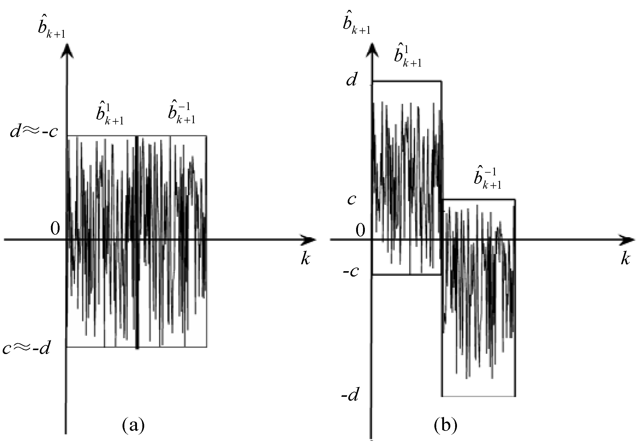
3.3. Blind Demodulation of CDS-SS Signals under Colored/Non-Gaussian Noises Condition

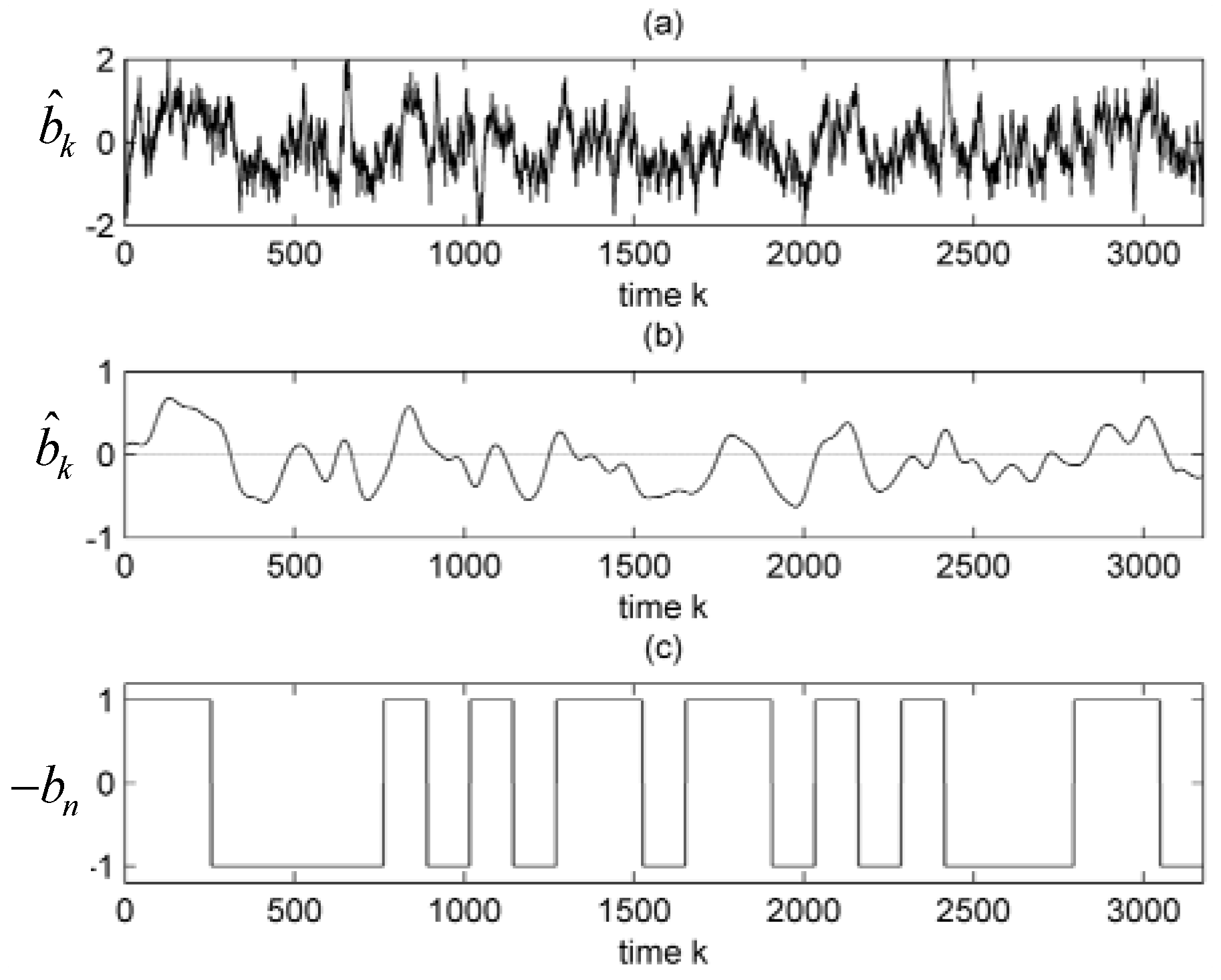
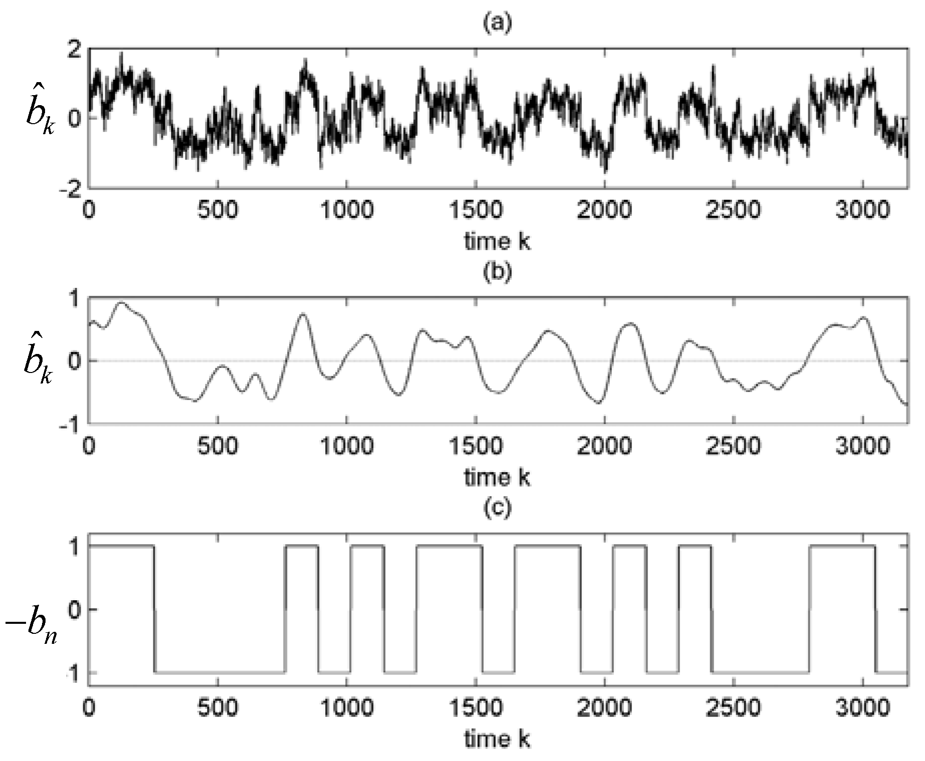
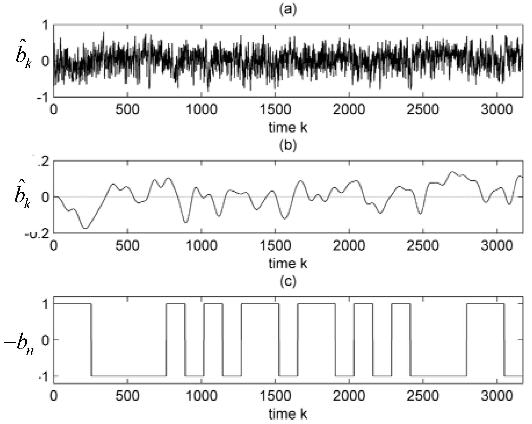
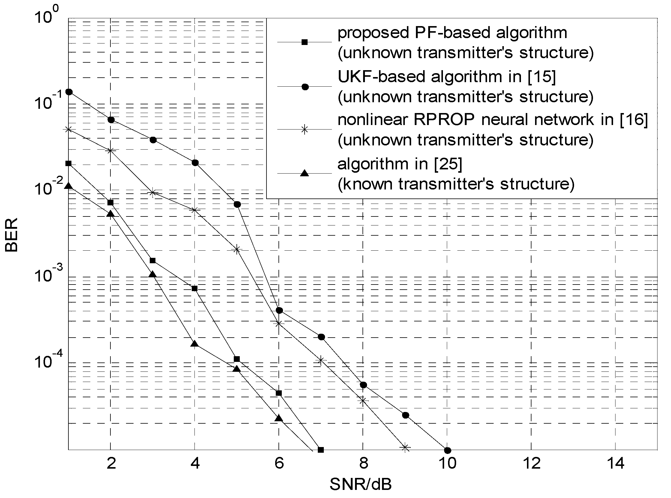
Under the condition that the noises is colored or non-Gaussian as described in Equations (15) and (16), the range-differentiating factor $\beta$ is imported into Equation (16) as shown in Equation (27):

$$\{\begin{array}{c}\begin{array}{l}{\overline{b}}_{k+1}=\left[\begin{array}{c}{\widehat{b}}_k\\ 0\end{array}\right]+\left[\begin{array}{c}{T}^{(2)}\\ {\tilde{A}}_2\end{array}\right]{\tilde{b}}_k+\left[\begin{array}{c}1\\ {\tilde{B}}_2\end{array}\right]n_k^{(2)}\\ =\left[\begin{array}{c}{\widehat{b}}_k\\ 0\end{array}\right]+{\overline{A}}_2{\tilde{b}}_k+{\overline{B}}_2{n}_k^{(2)}\end{array}\\ z_{k+1}={\widehat{b}}_{k+1}(g({\widehat{x}}_k)+\beta )+v_{k+1}^{(2)}\end{array}$$

(27)

Then, the proposed algorithm of alternately estimating the message signal $\left\{{\widehat{b}}_k\right\}$ and chaotic state $\left\{{\widehat{x}}_k\right\}$ according to Equations (15) and (27) by two PFs is illustrated in Figure 2 and described as follows.

Figure 2. Flow chart of the proposed PF-based algorithm.

Figure 2. Flow chart of the proposed PF-based algorithm.

(1) Initialization

Begin by generating samples ${\left\{{\overline{x}}_0^j\right\}}_{j=1}^M$ and ${\left\{{\overline{b}}_0^j\right\}}_{j=1}^M$ from their initial probabilities $p({\overline{x}}_0)$ and $p({\overline{b}}_0)$, respectively. Since the $p({\overline{x}}_0)$ and $p({\overline{b}}_0)$ are unknown, they can be assumed to be uniform distributions in bounded state spaces by making use of the limited range of the chaotic system. The algorithm starts from a random measure with equal weight on each of the M samples (M will always be 1,000 unless otherwise stated). Weight ${\lambda }_{\overline{x}}^j=1/M$, ${\lambda }_{\overline{b}}^j=1/M$;

(2) Estimate ${\widehat{b}}_{k+1}$ according to Equation (27) and ${\widehat{x}}_k$ (for $k=0,1,\mathrm{...}$). The state equation is ${\overline{b}}_{k+1}={\left[\begin{array}{cc}{\widehat{b}}_k& 0\end{array}\right]}^{\text{T}}+{\overline{A}}_2{\tilde{b}}_k+{\overline{B}}_2{n}_k^{(2)}$, and the measurement equation is $z_{k+1}={\widehat{b}}_{k+1}(g({\widehat{x}}_k)+\beta )+v_{k+1}^{(2)}$.

(2.1) Prediction/sampling step

Sample M values ${\left\{n_k^{(2),j}\right\}}_{j=1}^M$ from the probability density function of $n_k^{(2)}$, which is a white noise with known distribution. Then calculate:

$${\overline{b}}_{k+1|k}^j=\left[\begin{array}{c}{\widehat{b}}_k^j\\ 0\end{array}\right]+{\overline{A}}_2{\tilde{b}}_k^j+{\overline{B}}_2{n}_k^{(2),j}$$

(28)

Therefore, the prior probability function of ${\overline{b}}_{k+1}$ at time step k is approximated as:

$$p({\overline{b}}_{k+1}|z_{1:k})=\frac{1}{M}{\displaystyle {\sum }_{j=1}^M\delta ({\overline{b}}_{k+1|k}-{\overline{b}}_{k+1|k}^j)}$$

(29)

where $z_{1:k}=\{z_1,\mathrm{...},z_k\}$.

(2.2) Measurement update step

On receiving the measurement $z_{k+1}$, calculate the weight ${\overline{\lambda }}_{\overline{b}}^j$ by:

$${\overline{\lambda }}_{\overline{b}}^j=\frac{p_{v^{(2)}}(z_{k+1}-{\widehat{b}}_{k+1|k}^j(g({\widehat{x}}_k)+\beta ))}{{\displaystyle {\sum }_{j=1}^M{p}_{v^{(2)}}(z_{k+1}-{\widehat{b}}_{k+1|k}^j(g({\widehat{x}}_k)+\beta ))}}$$

(30)

where $p_{v^{(2)}}$ denotes the distribution of the measurement noise $v^{(2)}$ in Equation (27). Then the posterior probability density function is approximated as:

$$p({\overline{b}}_{k+1}|z_{1:k+1})={\displaystyle {\sum }_{j=1}^M{\overline{\lambda }}_{\overline{b}}^j\delta ({\overline{b}}_{k+1}-{\overline{b}}_{k+1|k}^j)}$$

(31)

and the estimation of ${\overline{b}}_{k+1}$ is:

$${\overline{b}}_{k+1}=E[{\overline{b}}_{k+1}|z_{1:k+1}]={\displaystyle {\sum }_{j=1}^M{\overline{\lambda }}_{\overline{b}}^j{\overline{b}}_{k+1}^j}$$

(32)

Then, the state ${\widehat{b}}_{k+1}$ is obtained from ${\overline{b}}_{k+1}={\left[\begin{array}{cc}{\widehat{b}}_{k+1}& {\tilde{b}}_{k+1}^T\end{array}\right]}^T$ directly;

(3) Estimate ${\widehat{x}}_{k+1}$ according to Equation (15) and ${\widehat{b}}_{k+1}$ (for $k=0,1,\mathrm{...}$). The state equation is ${\overline{x}}_{k+1}={\left[\begin{array}{cc}g({\widehat{x}}_k)& 0\end{array}\right]}^{\text{T}}+{\overline{A}}_1{\tilde{x}}_k+{\overline{B}}_1{n}_k^{(1)}$, and the measurement equation is $z_{k+1}=\mathrm{sgn}({\widehat{b}}_{k+1}){\widehat{x}}_{k+1}+v_{k+1}^{(1)}$.

(3.1) Prediction/sampling step

Sample M values ${\left\{n_k^{(1),j}\right\}}_{j=1}^M$ from the probability density function of $n_k^{(1)}$, which is a white noise with known distribution. Then calculate:

$${\overline{x}}_{k+1|k}^j=\left[\begin{array}{c}g({\widehat{x}}_k^j)\\ 0\end{array}\right]+{\overline{A}}_1{\tilde{x}}_k^j+{\overline{B}}_1{n}_k^{(1),j}$$

(33)

Therefore, the prior probability function of ${\overline{x}}_{k+1}$ at time step k is approximated as:

$$p({\overline{x}}_{k+1}|z_{1:k})=\frac{1}{M}{\displaystyle {\sum }_{j=1}^M\delta ({\overline{x}}_{k+1|k}-{\overline{x}}_{k+1|k}^j)}$$

(34)

(3.2) Measurement update step

On receiving the measurement $z_{k+1}$, calculate the weight ${\overline{\lambda }}_{\overline{x}}^j$ by:

$${\overline{\lambda }}_{\overline{x}}^j=\frac{p_{v^{(1)}}(z_{k+1}-\mathrm{sgn}({\widehat{b}}_{k+1}){\widehat{x}}_{k+1|k}^j)}{{\displaystyle {\sum }_{j=1}^M{p}_{v^{(1)}}(z_{k+1}-\mathrm{sgn}({\widehat{b}}_{k+1}){\widehat{x}}_{k+1|k}^j)}}$$

(35)

where $p_{v^{(1)}}$ denotes the distribution of the measurement noise $v^{(1)}$ in Equation (15). Then the posterior probability density function of ${\overline{x}}_{k+1}$ is expressed as follows:

$$p({\overline{x}}_{k+1}|z_{1:k+1})={\displaystyle {\sum }_{j=1}^M{\overline{\lambda }}_{\overline{x}}^j\delta ({\overline{x}}_{k+1}-{\overline{x}}_{k+1|k}^j)}$$

(36)

and the estimation of ${\overline{x}}_{k+1}$ is:

$${\overline{x}}_{k+1}=E[{\overline{x}}_{k+1}|z_{1:k+1}]={\displaystyle {\sum }_{j=1}^M{\overline{\lambda }}_{\overline{x}}^j{\overline{x}}_{k+1}^j}$$

(37)

Then, the state ${\widehat{x}}_{k+1}$ is obtained from ${\overline{x}}_{k+1}={\left[\begin{array}{cc}{\widehat{x}}_{k+1}& {\tilde{x}}_{k+1}^T\end{array}\right]}^{\text{T}}$ directly;

(4) Resampling step

The resulting particles ${\left\{{\overline{x}}_{k+1}^j\right\}}_{j=1}^M$ and ${\left\{{\overline{b}}_{k+1}^j\right\}}_{j=1}^M$ satisfy the posterior probability density functions $p({\overline{x}}_{k+1}|z_{1:k+1})$ and $p({\overline{b}}_{k+1}|z_{1:k+1})$, respectively. The particles with different weights are replaced with new ones having equal weights (1/M);

(5) Iteration step

Let $k=k+1$ go to step (ii). To recover the original binary message $b_n$, the estimated messages $\left\{{\widehat{b}}_k\right\}$ are lowpass filtered, and then the ${\widehat{b}}_k$ is binary quantized as ${\widehat{b}}_n$. Usually, ${\widehat{b}}_n=-b_n$, which will not affect extracting the binary message.

4. Simulations

In this section, the famous Logistic map is illustrated to verify the effectiveness of the proposed algorithm. The transmitter’s chaotic sequence is generated by the Logistic map:

$$x_{k+1}=f(x_k)=1-2x_k^2$$

(38)

In [28], it is proved and demonstrated that the tent map can obtain generalized synchronization with the Logistic map even on a condition of a weak coupling. In this research, it is a strong coupling, so an intruder can use the tent map to fit the transmitter’s chaotic map.

The tent map is:

$$x_{k+1}=g(x_k)=0.5-1.99\left|x_k\right|$$

(39)

Suppose that the colored non-Gaussian process noises $w_k^{(1)}$ and $w_k^{(2)}$ satisfy:

$$w_k^{(1)}-1.5w_{k-1}^{(1)}+0.8w_{k-2}^{(1)}=n_k^{(1)}-0.75n_{k-1}^{(1)}-2.5n_{k-2}^{(1)}$$

(40)

$$w_k^{(2)}=n_k^{(2)}-n_{k-1}^{(2)}+0.2n_{k-2}^{(2)}$$

(41)

where the white non-Gaussian noises $n_k^{(1)}$ and $n_k^{(2)}$ are obey the exponential distributions $p_{n^{(1)}}(n_k^{(1)})=25\exp (-25n_k^{(1)})$ and $p_{n^{(2)}}(n_k^{(2)})=20\exp (-20n_k^{(2)})$, respectively. It should be mentioned that the distribution of the noises is obtained by the priori knowledge in practice.

Assume that the measurement noises $v_k^{(1)}$ and $v_k^{(2)}$ with zero-mean and arbitrary distribution are both white Gaussian noises for simplicity, the spreading factor N is 127, and the range-differentiating factor $\beta$ is 0.9.

Figure 3 shows the estimated message ${\widehat{b}}_k$ without the range-differentiating factor at a signal-to-noise ratio (SNR) of 7dB, i.e., $\beta =0$, from which the message symbols cannot be recovered because the values of ${\widehat{b}}_k^1$ and ${\widehat{b}}_k^{-1}$ vibrate in the same range.

Figure 3. (a) The estimated message ${\widehat{b}}_k$ when $\beta =0$ at SNR = 7dB; (b) the result of lowpass filtering; (c) the original transmitted binary message $-b_n$.

Figure 3. (a) The estimated message ${\widehat{b}}_k$ when $\beta =0$ at SNR = 7dB; (b) the result of lowpass filtering; (c) the original transmitted binary message $-b_n$.

Hu and Guo [15] proposed a modified UKF to blindly demodulate the CDS-SS signals accurately under the white Gaussian noises condition. However, in the case of colored noises in Equations (40) and (41), errors appear as shown in Figure 4.

Figure 4. (a) The message ${\widehat{b}}_k$ estimated by UKF when $\beta =0.9$ at SNR = 7dB; (b) the result of lowpass filtering; (c) the original transmitted binary message $-b_n$.

Figure 4. (a) The message ${\widehat{b}}_k$ estimated by UKF when $\beta =0.9$ at SNR = 7dB; (b) the result of lowpass filtering; (c) the original transmitted binary message $-b_n$.

Figure 4(a) shows the message ${\widehat{b}}_k$ estimated by UKF at SNR = 7dB; Figure 4(b) shows the result of lowpass filtering; Figure 4(c) shows the original transmitted binary message $-b_n$.

In [5], under a condition of cooperative communication (known transmitter structure), several data blocks containing up to 200 bits were transmitted at a SNR of about 7–8 dB, and no error was noticed at the authorized receiver. In this paper, under the conditions of non-cooperative communication (unknown transmitter structure) and colored or non-Gaussian noises, the intercepted CDS-SS signals containing 200 bits at SNR = 7 dB are blindly demodulated by the proposed PF-based algorithm, and no error is found. Figure 5(a) shows the message ${\widehat{b}}_k$ estimated by PF at SNR = 7dB; Figure 5(b) shows the result of lowpass filtering; Figure 5(c) shows the original transmitted binary message $-b_n$.

Figure 5. (a) The message ${\widehat{b}}_k$ estimated by PF when $\beta =0.9$ at SNR = 7dB; (b) the result of lowpass filtering; (c) the original transmitted binary message $b_n$.

Figure 5. (a) The message ${\widehat{b}}_k$ estimated by PF when $\beta =0.9$ at SNR = 7dB; (b) the result of lowpass filtering; (c) the original transmitted binary message $b_n$.

In [25], the PF is used to estimate the parameter of the chaotic system with the requirement that the structure of the chaotic map is known. For comparison in the simulation, the algorithm in [25] is also modified by the fact that the colored or non-Gaussian noises are formulated by ARMA models, and then the parameters that model the noises are included in the state vector. A nonlinear RPROP neural network is developed to blindly demodulate (unknown transmitter structure) the CDS-SS signals in [16]. Figure 6 gives the bit-error rate (BER) performances of the algorithm in [25], the nonlinear RPROP neural network algorithm in [16], the UKF-based algorithm in [15] and the proposed PF-based algorithm with the noises in Equations (40) and (41). The BER of the proposed algorithm is about ${10}^{-5}$ at SNR = 7dB. It can be concluded that the BER performance of the proposed PF-based algorithm is better than the nonlinear RPROP neural network and the UKF-based algorithm on the non-cooperative communication condition (unknown transmitter’s structure), and approaches the level the algorithm in [25] that is belong to the cooperative communication (known transmitter’s structure) could achieve.

Figure 6. Comparison of BER performance among the algorithm in [25], the nonlinear RPROP neural network algorithm in [16], the UKF-based algorithm in [15] and the proposed PF-based algorithm.

Figure 6. Comparison of BER performance among the algorithm in [25], the nonlinear RPROP neural network algorithm in [16], the UKF-based algorithm in [15] and the proposed PF-based algorithm.

5. Conclusions

In order to blindly demodulate the CDS-SS signals under the colored or non-Gaussian noises condition, a PF-based algorithm is proposed in this paper. To implement this algorithm, the intruder uses a different chaotic system equation to fit the transmitter’s chaotic system equation. Moreover, the colored or non-Gaussian noises are formulated by ARMA models. In addition, the range-differentiating factor is imported into the intruder’s chaotic system equation. Therefore, two modified PFs are obtained, which are implemented in reciprocal interaction to estimate the message and the chaotic state. Since the range-differentiating factor is able to make the inevitable chaos fitting error advantageous, the CDS-SS signals can be blindly demodulated according to the range of the estimated message signals. Simulations show that the proposed algorithm is robust to both colored or non-Gaussian noises, and the original binary message can be retrieved from the CDS-SS signals with satisfactory BER performance without any knowledge of the transmitter’s chaotic map, parameters, or initial value.

References

1. Alvarez, G.; Montoya, F.; Romera, M.; Pastor, G. Breaking two secure communication systems based on chaotic masking. IEEE Trans. Circuits Syst. II Express Briefs 2004, 51, 505–506. [Google Scholar] [CrossRef]
2. Yang, T.; Yang, L.B.; Yang, C.M. Breaking chaotic switching using generalized synchronization: Examples. IEEE Trans. Circuits Syst. I Fundam. Theory Appl. 1998, 45, 1062–1067. [Google Scholar] [CrossRef]
3. Alvarez, G.; Montoya, F.; Romera, M.; Pastor, G. Breaking parameter modulated chaotic secure communication system. Chaos Soliton. Fract. 2004, 21, 783–787. [Google Scholar] [CrossRef]
4. Parlitz, U.; Ergezinger, S. Robust communication based on chaotic spreading sequences. Phys. Lett. A 1994, 188, 146–150. [Google Scholar] [CrossRef]
5. Azou, S.; Pistre, C.; Duff, L.L.; Burel, G. Sea Trial Results of a Chaotic Direct-Sequence Spread Spectrum Underwater Communication System. In Proceedings of IEEE-OCEANS’03, San Diego, CA, USA, September 2003; pp. 1539–1546.
6. Hwang, Y.; Papadopoulos, H.C. Physical-layer secrecy in AWGN via a class of chaotic DS/SS systems: Analysis and design. IEEE Trans. Signal Process. 2004, 52, 2637–2649. [Google Scholar] [CrossRef]
7. Yu, J.; Yao, Y.D. Detection performance of chaotic spreading LPI waveforms. IEEE Trans. Wireless Commun. 2005, 4, 390–396. [Google Scholar]
8. Sameh, M.; Ali, S.T.; Naceur, B.B. Particle Filter for State and Unknown Input Estimation of Chaotic Systems. In Proceedings of International Conference on Control, Engineering and Information Technology, Nanning, China, August 2013; pp. 67–72.
9. Chen, M.; Min, W. Unknown input observer based chaotic secure communication. Phys. Lett. A 2008, 372, 1595–1600. [Google Scholar] [CrossRef]
10. Dimassi, H.; Loría, A. Adaptive unknown-input observers-based synchronization of chaotic systems for telecommunication. IEEE Trans. Circuits Syst. I Regul. Pap. 2011, 58, 800–812. [Google Scholar] [CrossRef] [Green Version]
11. Park, S.; Hwang, J.P.; Kim, E. A new state estimation method for chaotic signals: Map-particle filter method. Expert Syst. Appl. 2011, 38, 11442–11446. [Google Scholar] [CrossRef]
12. Xu, Y.; Zhou, W.; Fang, J.; Sun, W. Adaptive bidirectionally coupled synchronization of chaotic systems with unknown parameters. Nonlinear Dyn. 2011, 66, 67–76. [Google Scholar] [CrossRef]
13. Li, X.F.; Chi, S.L.A.; Han, X.P.; Liu, X.J.; Chu, Y.D. Complete (anti-)synchronization of chaotic systems with fully uncertain parameters by adaptive control. Nonlinear Dyn. 2011, 63, 263–275. [Google Scholar] [CrossRef]
14. Aghababa, M.P.; Akbari, M.E. A chattering-free robust adaptive sliding mode controller for synchronization of two different chaotic systems with unknown uncertainties and external disturbances. Appl. Math. Comput. 2012, 218, 5757–5768. [Google Scholar] [CrossRef]
15. Hu, J.F.; Guo, J.B. Breaking a chaotic direct sequence spreading spectrum secure communication system. Acta Phys. Sin. 2008, 57, 1477–1484. [Google Scholar]
16. Hu, J.F.; Guo, J.B. Blind estimation of chaotic spread spectrum sequences. J. Electr. Inform. Technol. 2008, 30, 1824–1827. [Google Scholar] [CrossRef]
17. Xu, X.Z.; Guo, J.B. A novel unified equalization and demodulation of chaotic direct sequence spreading spectrum signal based on state estimation. Acta Phys. Sin. 2011, 60, e020510. [Google Scholar]
18. Alvarez, G.; Montoya, F.; Pastor, G.; Romera, M. Breaking a secure communication scheme based on the phase synchronization of chaotic systems. Chaos 2004, 14, 274–278. [Google Scholar] [CrossRef] [PubMed] [Green Version]
19. Luca, M.B.; Azou, S.; Hodina, E.; Serbanescu, A.; Burel, G. Pseudoblind Demodulation of Chaotic DS-SS Signals through Exact Kalman Filtering. In Proceedings of IEEE Communications Conference, Bucharest, Romania, June 2006; pp. 1–4.
20. Yang, T.; Yang, L.B.; Yang, C.M. Breaking chaotic secure communication using a spectrogram. Phys. Lett. A 1998, 247, 105–109. [Google Scholar] [CrossRef]
21. Hu, G.J.; Feng, Z.J.; Meng, R.L. Chosen ciphertext attack on chaos communication based on chaotic synchronization. IEEE Trans. Circuits Syst. I Fundam. Theory Appl. 2003, 50, 275–279. [Google Scholar]
22. Gordon, N.J.; Salmond, D.J.; Smith, A.F.M. Novel approach to nonlinear/non-Gaussian Bayesian state estimation. Proc. Ins. Electr. Eng. 1993, 140, 107–113. [Google Scholar] [CrossRef]
23. Shi, Z.G.; Hong, S.H.; Chen, J.M.; Chen, K.S.; Sun, Y.X. Particle filter-based synchronization of chaotic colpitts circuits combating AWGN channel distortion. Circuits Syst. Signal Process. 2008, 27, 833–845. [Google Scholar] [CrossRef]
24. Watzenig, D.; Brandner, M.; Steiner, G. A particle filter approach for tomographic imaging based on different state-space representations. Meas. Sci. Technol. 2007, 18, 30–40. [Google Scholar] [CrossRef]
25. Li, H.; Feng, S.F. Parameter modulated chaotic communication based on particle fitler. J. Comput. Inform. Syst. 2008, 7, 4417–4424. [Google Scholar]
26. Zhang, B.; Chen, M.Y.; Zhou, D.H.; Li, Z.X. Particle-filter-based estimation and prediction of chaotic states. Chaos Solition. Fract. 2007, 32, 1491–1498. [Google Scholar] [CrossRef]
27. Grewal, M.S.; Andrews, A.P. Nonlinear filtering. In Kalman Filtering: Theory and Practice Using Matlab, 2nd ed.; Wiley: New York, NY, USA, 2001; pp. 289–314. [Google Scholar]
28. Afraimovich, V.; Cordonet, A.; Rulkov, N.F. Generalized synchronization of chaos in noninvertible maps. Phys. Rev. E 2002, 66, e016208. [Google Scholar] [CrossRef]