Article

SpaGrOW—A Derivative-Free Optimization Scheme for Intermolecular Force Field Parameters Based on Sparse Grid Methods

1
Fraunhofer Institute for Algorithms and Scientific Computing (SCAI), Schloss Birlinghoven, Sankt Augustin 53757, Germany
2
Hochschule-Bonn Rhein-Sieg (HBRS), Grantham-Allee 20, Sankt Augustin 53757, Germany
*
Author to whom correspondence should be addressed.
Entropy 2013, 15(9), 3640-3687; https://doi.org/10.3390/e15093640
Submission received: 16 February 2013 / Revised: 15 July 2013 / Accepted: 28 August 2013 / Published: 6 September 2013
(This article belongs to the Special Issue Molecular Dynamics Simulation)

Abstract

:
Molecular modeling is an important subdomain in the field of computational modeling, regarding both scientific and industrial applications. This is because computer simulations on a molecular level are a virtuous instrument to study the impact of microscopic on macroscopic phenomena. Accurate molecular models are indispensable for such simulations in order to predict physical target observables, like density, pressure, diffusion coefficients or energetic properties, quantitatively over a wide range of temperatures. Thereby, molecular interactions are described mathematically by force fields. The mathematical description includes parameters for both intramolecular and intermolecular interactions. While intramolecular force field parameters can be determined by quantum mechanics, the parameterization of the intermolecular part is often tedious. Recently, an empirical procedure, based on the minimization of a loss function between simulated and experimental physical properties, was published by the authors. Thereby, efficient gradient-based numerical optimization algorithms were used. However, empirical force field optimization is inhibited by the two following central issues appearing in molecular simulations: firstly, they are extremely time-consuming, even on modern and high-performance computer clusters, and secondly, simulation data is affected by statistical noise. The latter provokes the fact that an accurate computation of gradients or Hessians is nearly impossible close to a local or global minimum, mainly because the loss function is flat. Therefore, the question arises of whether to apply a derivative-free method approximating the loss function by an appropriate model function. In this paper, a new Sparse Grid-based Optimization Workflow (SpaGrOW) is presented, which accomplishes this task robustly and, at the same time, keeps the number of time-consuming simulations relatively small. This is achieved by an efficient sampling procedure for the approximation based on sparse grids, which is described in full detail: in order to counteract the fact that sparse grids are fully occupied on their boundaries, a mathematical transformation is applied to generate homogeneous Dirichlet boundary conditions. As the main drawback of sparse grids methods is the assumption that the function to be modeled exhibits certain smoothness properties, it has to be approximated by smooth functions first. Radial basis functions turned out to be very suitable to solve this task. The smoothing procedure and the subsequent interpolation on sparse grids are performed within sufficiently large compact trust regions of the parameter space. It is shown and explained how the combination of the three ingredients leads to a new efficient derivative-free algorithm, which has the additional advantage that it is capable of reducing the overall number of simulations by a factor of about two in comparison to gradient-based optimization methods. At the same time, the robustness with respect to statistical noise is maintained. This assertion is proven by both theoretical considerations and practical evaluations for molecular simulations on chemical example substances.

1. Introduction

In the last few decades, computer simulations have gained in importance for both science and industry, particularly due to the fast development of parallel high performance clusters. A denotative subarea of computer simulations are molecular simulations, which allow one to study the effects of modifications in microscopic states on macroscopic system properties. In contrast to simulations in process engineering, not the continuum, but the molecular level of a system is modeled. Thereby, the goal is to describe interatomic and intermolecular interactions, so that, on the one hand, certain accuracy demands are fulfilled, and on the other hand, the required computation time is as low as possible. The latter aspect is very important, because molecular simulations are numerically costly, also on modern computer clusters. The industrial relevance of molecular simulations originates from the fact that labor- and cost-intensive chemical experiments can be avoided. Hence, chemical systems can be simulated at temperatures and pressures that are very difficult to realize in a laboratory, the properties of toxic substances can be calculated without any risk and measure of precaution and processes on surfaces or within membranes are observable on a microscopic level. Another advantage of molecular simulations is that both the location and velocity of each particle are saved after certain time intervals, which results in a detailed observation of the behavior of the system. Altogether, molecular simulations have emerged as their own scientific discipline, and because of the continuous growth of computer resources, they will still become much more important in the coming years [1,2].
In principle, it is possible to describe interactions within a chemical system by quantum mechanics. Thereby, a partial differential equation, the so-called Schrödinger equation [3], has to be solved. As this turns out to be extremely difficult, especially for multi-particle systems, the problem is simplified by classical mechanical methods. Then, the system is considered on an atomistic level, i.e., the smallest unit is an atom. Molecular simulation techniques are based on statistical mechanics, a subarea of classical mechanics. The most important simulation methods are molecular dynamics (MD) and Monte Carlo (MC). Thereby, both intra- and inter-molecular interactions are described by the foundation of a simulation, the force field. A force field consists of an analytic term and parameters to be adjusted. It is given by the potential energy, which has the following typical form [1,4]:
U pot ( r M ) : = Bonds k r 2 r - r 0 2 + Angles k ϕ 2 ϕ - ϕ 0 2 + Dihedrals n = 1 m V n cos ( n ω )
+ i < j N 4 ε i j σ i j r i j 12 - σ i j r i j 6 + q i q j 4 π ε 0 r i j
Thereby, r M R 3 M is a vector containing all three-dimensional coordinates of the interaction sites, where M is the number of particles in the system. The first row of Equation (1) describes the intramolecular and the second row the intermolecular part. The parameters of the intramolecular part, modeling the interactions caused by the modifications of bond lengths r, bond angles ϕ and dihedral angles ω can be computed by quantum mechanics. Please note that the index, 0 , denotes the respective parameter in equilibrium and that k r and k ϕ are force constants. The factors, V n , n = 1 , . . . , m , m N , describe the rotation barriers around the molecular axes. The parameterization of the intermolecular part, modeling the interactions caused by dispersion—described by the Lennard-Jones (LJ) parameters, σ i j and ε i j , i , j = 1 , . . . , M , i < j , and electrostatic effects—described by partial atomic charges, q i and q j , i , j = 1 , . . . , M , i < j , is often tedious. The constant, ε 0 = 8 . 854 × 10 - 12 Fm - 1 , is the dielectric constant.

1.1. Force Field Parameterization

It is known from the literature that many force fields describe molecular interactions accurately, qualitatively and quantitatively [5]. Intramolecular parameters can be determined by quantum mechanics, i.e., by the minimization of a potential hyperplane. Partial atomic charges can also be computed from the position of nuclei and electrons. However, quantum mechanical methods require a high computational effort, especially for large molecules. This is why some simplifications were carried out, and the adjustment of the parameters was performed by fitting them to spectroscopic data. Some of the most famous force fields based on such semiempirical methods have been developed, e.g., by [6,7,8]. Quantum mechanical calculations of partial atomic charges were realized, e.g., by [9]. In related work [10,11], the automized optimization workflow, WOLF 2 PACK, was created, which combines quantum mechanical algorithms with atomistic models and is capable of calculating both optimal intramolecular force field parameters and partial atomic charges. For the intermolecular part of Equation (1), the respective force field parameters were mostly adjusted to experimental target data, i.e., physical properties resulting from a molecular simulation were compared with experimental reference data. In particular, this empirical approach was realized by [12,13,14]. However, the parameters obtained cannot be considered as optimal, because they were not fitted to a large number of experimental data. Furthermore, in most cases, they ware adjusted manually, which is always time-consuming. They are transferable to other substances, but a subsequent readjustment is indispensable [15]. Many users take standard force fields from the literature for their simulations, which may lead to satisfactory, but not to optimal, target properties.
In the last decade, a few approaches were published realizing an automated force field parameterization procedure [16,17,18,19,20]. Thereby, physical target properties, like density, enthalpy of vaporization and vapor pressure, were fitted to their respective experimental reference data at different temperatures and pressures simultaneously. This was done via the minimization of a quadratic loss function between simulated and experimental data, i.e., by solving a mathematical optimization problem with numerical optimization algorithms. This approach is pursued in this paper, as well. The loss function to be minimized is given by:
F : R N R 0 +
x i = 1 n w i 2 f i exp - f i sim ( x ) f i exp 2
where x = ( x 1 , . . . , x N ) T is a force field parameter vector, N the dimension of the parameter space, n the number of considered physical properties, maybe at different temperatures, f i sim ( x ) , i = 1 , . . . , n the simulated physical target properties as functions of the parameter vector, x, and f i exp , i = 1 , . . . , n the respective experimental reference data. The weights, w i 2 , i = 1 , . . . , n , account for the fact that some properties are easier to reproduce or measured more accurately than others. The loss function, F, is minimized within a compact domain, Ω R N .
The optimization workflow is shown in Figure 1: the initial guess has to be reasonably close to the minimum. The target properties computed by a simulation tool are inserted into loss function in Equation (3) and compared with the experimental target properties. If a specified stopping criterion is fulfilled, the parameters are final, and the workflow terminates. Otherwise, the current parameter vector is passed on to the optimization procedure searching for new parameters with a lower loss function value.
There are two main requirements for the numerical optimization algorithms solving the minimization problem: Firstly, they have to be efficient, i.e., their convergency must be fast and the number of function evaluations has to be low, because for each function evaluation, time-consuming molecular simulations are needed, which can be parallelized for the different temperatures. Secondly, they have to be robust with respect to statistical noise, because simulation data is always affected by uncertainties. The reason for this is the fact that physical properties are computed by averaging over a certain time period in the case of MD simulations and over a certain number of system states in the case of MC simulations. In previous work [21,22,23], the software package, Gradient-based Optimization Workflow (GROW), was developed. Thereby, efficient gradient-based numerical optimization algorithms were successfully applied to minimize loss function in Equation (3) in an efficient and robust way. Thereby, simple methods, like steepest descent and conjugate gradient algorithms, turned out to be most suitable. Algorithms requiring a Hessian were too time-consuming or not reliable whenever the Hessian was assumed to be positive definite, which it was not in most cases. Gradients and Hessians were approximated using first-order finite differences. The lengths of the descent directions were computed by an Armijo step length control mechanism.
Figure 1. Optimization workflow: The target properties are computed for an initial guess for the force field parameters. If they do not agree sufficiently well with the experimental target properties, the optimization procedure is performed searching for new parameters with a lower loss function value.
Entropy 15 03640 g001
However, the accurate computation of a gradient or a Hessian is problematic close to a global or local minimum of F, due to the presence of statistical noise, cf. Figure 2. For the finite difference approximation of the gradient, two adjacent points are necessary. If these two points are situated too close to each other, their loss function values cannot be distinguished anymore, due to the error bars surrounding them. Therefore, the direction of the approximated gradient can be completely wrong. This leads to the motivation to develop a new efficient derivative-free method counteracting this problem. The right side of Figure 2 shows that a possible solution is to approximate the loss function by an adequate model function and to determine the minimum of the model function. In this work, a new Sparse Grid-based Optimization Workflow (SpaGrOW) is presented in detail, implementing the aforesaid modeling approach. The main difficulty is to filter out the statistical noise during the approximation process, which is realized in SpaGrOW by regularization methods. As approximation is always based on sampling the parameter space and as molecular simulations are required for all selected points within the sampling process, sparse grids are involved in order to avoid high computational effort. The combination technique developed by [24] is applied in order to perform a piecewise multilinear interpolation from a sparse grid to a full grid. As sparse grids are fully occupied at their boundaries, the loss function is artificially set to zero at the boundary by a mathematical transformation. Then, the minimum on the full grid is determined, and a back-transformation is performed. As the combination technique requires certain smoothness properties, and as the loss function cannot be assumed to be smooth, it has to be preprocessed. Hence, it is approximated by a smooth model function before. The selection of a suitable model function is done by both theoretical considerations and practical evaluations.
Figure 2. Motivation of a derivative-free method in the case of noisy loss function values close to the minimum; the direction of a gradient can be completely wrong. Hence, an approximation of the loss function is necessary. This regression procedure has to filter out the statistical noise.
Entropy 15 03640 g002
Another very important goal of SpaGrOW is to outperform gradient-based optimization algorithms with respect to computational effort, i.e., the number of molecular simulations to be performed should be reduced by about a factor of two. At the same time, it should be at least as robust as gradient-based methods. Hence, SpaGrOW should also be applicable in domains that are further away from the minimum. This can only be realized efficiently by a local consideration. The minimization of SpaGrOW is performed in a small compact trust region. As the minimum can be situated at the boundary of the trust region, the method becomes an iterative procedure. The actual minimum is accepted as a new iteration, if the piecewise multilinear model predicts the decreasing trend of the loss function in a reliable way. Hence, SpaGrOW is combined with the approach of another category of optimization algorithms, the Trust Region methods, cf. [25,26]. The speed of convergency can be controlled by the size of the trust region. Altogether, SpaGrOW is shown to be an efficient combination of numerical methods, which has the following three very important issues: it is efficient, robust and gets very close to the minimum, if certain assumptions are fulfilled. However, these assumptions cannot be proven a priori, because the shape of the loss function and the amount of statistical noise is unknown in most cases. Therefore, a detailed practical evaluation is indispensable.
The methodology of SpaGrOW is presented in detail in Section 2, including complexity and convergency considerations. Section 4 shows the results of a detailed practical evaluation of the methodology, and finally, Section 5 concludes the paper.

1.2. Drawbacks of Gradient-Based Methods

Although gradient-based optimization methods turned out to be suitable and also efficient instruments for the parameterization of force fields in previous work [21,22,23], they unfortunately have the following disadvantages:
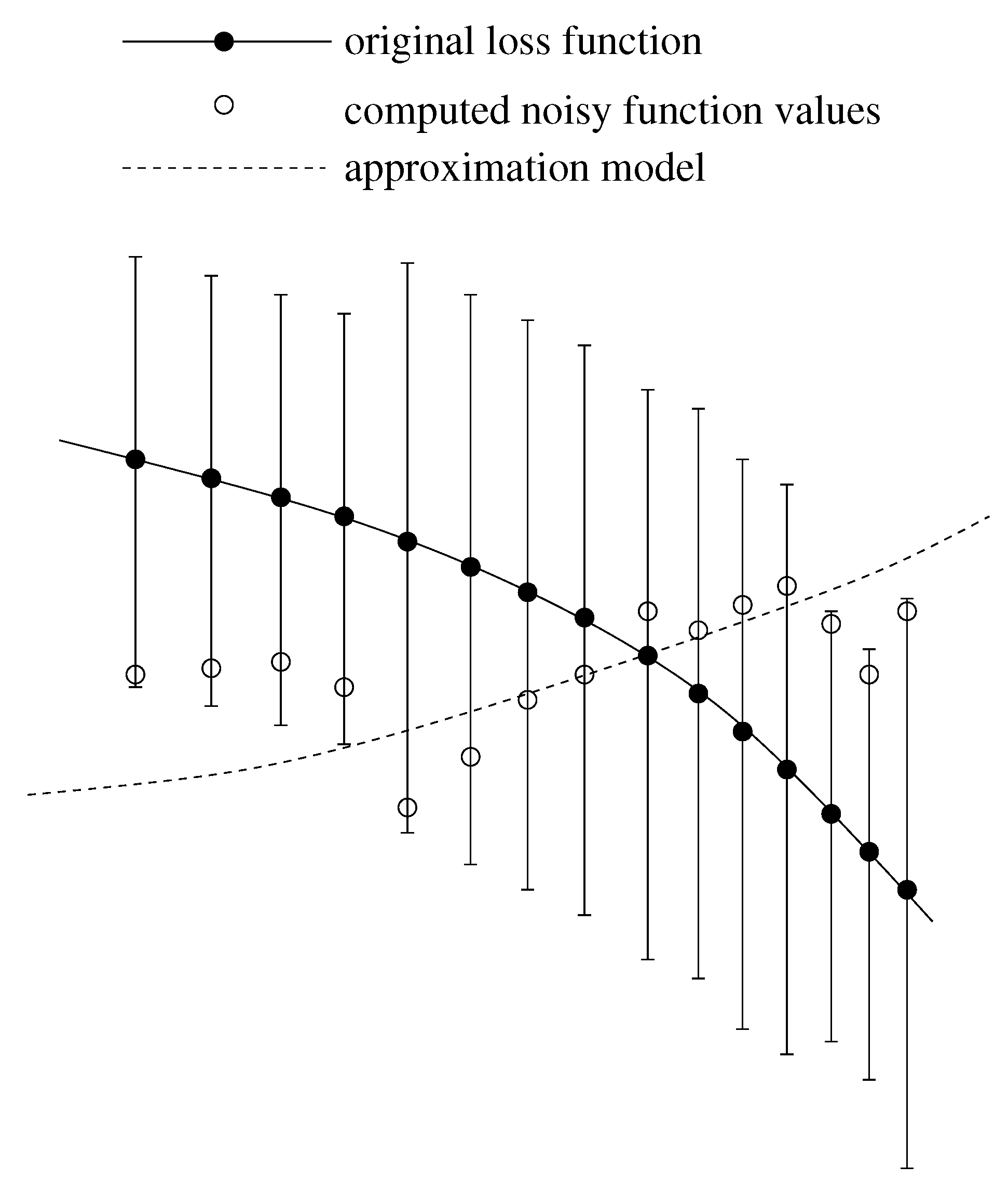
  • Due to the statistical noise in the simulation data, the accuracy of a gradient is always limited. It can only predict the decreasing trend of the loss function. As motivated above, this becomes problematic close to the minimum. Theoretically, it is possible to counteract this problem by a suitable discretization for the calculation of the finite differences. However, optimizing the distance of two adjacent points would lead to much more computational effort. Moreover, even if the direction of the gradient can be calculated accurately, the step length control algorithm will only deliver insignificantly small improvements compared to the higher amount of computation time. This is a drawback of the Armijo step length control, but the application of more efficient step length control mechanisms would lead to more computational effort again.
  • Whenever a descent direction is incorrect, a point with a smaller loss function value can only be found by chance, because there is no possibility to change the direction. In contrast to descent methods, Trust Region methods decrease the step length in order to find a new, maybe more suitable descent direction of the loss function. This is why these methods are able to get closer to the minimum. However, the Trust Region method applied in previous work requires a Hessian matrix, which leads to significantly more loss function evaluations.
  • The amount of simulations is still quite high for gradient- and especially Hessian-based optimization algorithms. At each iteration, a gradient or, additionally, a Hessian have to be computed, which leads to N or, even, N + N ( N + 1 ) / 2 loss function evaluations. Furthermore, the Armijo step length control algorithm requires additional functional evaluations.
These drawbacks of gradient-based methods motivate the development of an algorithm that is capable of both getting robustly closer to the minimum and solving the optimization problem with significantly less simulations. It should not assume the loss function to be smooth. Instead, it should use smoothing and regularization procedures in order to handle the statistical noise and jagged functions.

2. SpaGrOW Methodology: The Main Elements

In this work, a new derivative-free algorithm based on sparse grids and smoothing methods is presented. Figure 3 visualizes the gain in both efficiency and robustness by the combination of the Trust Region approach with the interpolation on sparse grids and smoothing procedures: the interpolation from a sparse grid to a full grid realizes a significant reduction of function evaluations, i.e., simulations, without increasing the interpolation error significantly, on the other hand. At each iteration, the loss function is smoothed before the interpolation is carried out. The quality of the interpolation model is measured following the Trust Region idea. The actual minimum, which is determined on the full grid, is either accepted as a new iteration or the trust region is decreased. It is desisted from a continuous minimization within the trust region in order to avoid additional internal optimization iterations. There also exist approaches to determine the global minimum of a piecewise-linearly interpolated function via so-called subgradients [27]. However, only for the interpolation itself, at least 3 N function evaluations are required. In the present case, there are constraints, due to the minimization on a compact trust region. Hence, the sparse grid approach seems to be more reasonable. Another advantage of the Trust Region approach is the fact that it is able to be fast at the beginning of the optimization procedure and to jump over undesired intermediate local minima. This is due to the size of the step length, which is selected before a descent direction is calculated.
Figure 3. Overview of the Sparse Grid-based Optimization Workflow (SpaGrOW): the combination of the Trust Region approach with the interpolation on sparse grids requiring a smoothing procedure to be preceded leads to both increasing efficiency and robustness.
Entropy 15 03640 g003
First, the two main elements of SpaGrOW are presented: In Section 2.1, the idea of sparse grids is introduced and the advantages with respect to reduction of computation time are presented. Suitable smoothing and regularization procedures are described in Section 2.2. The algorithm of SpaGrOW is introduced afterwards in Section 3.

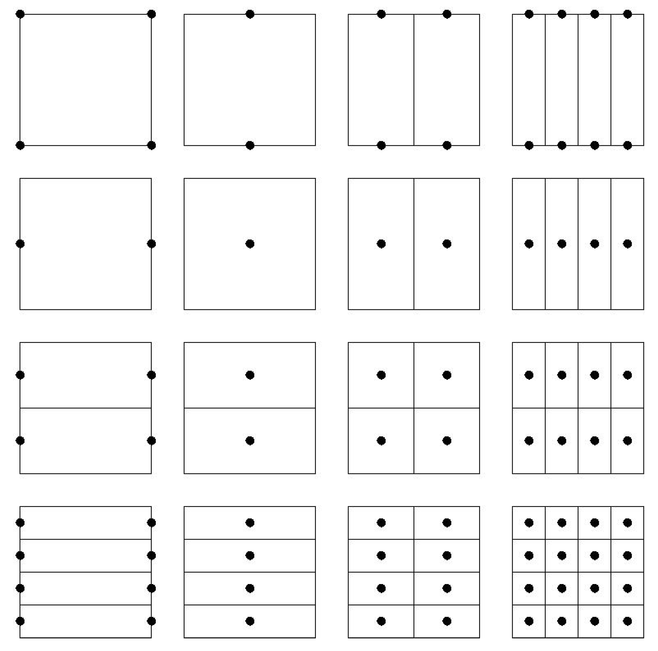
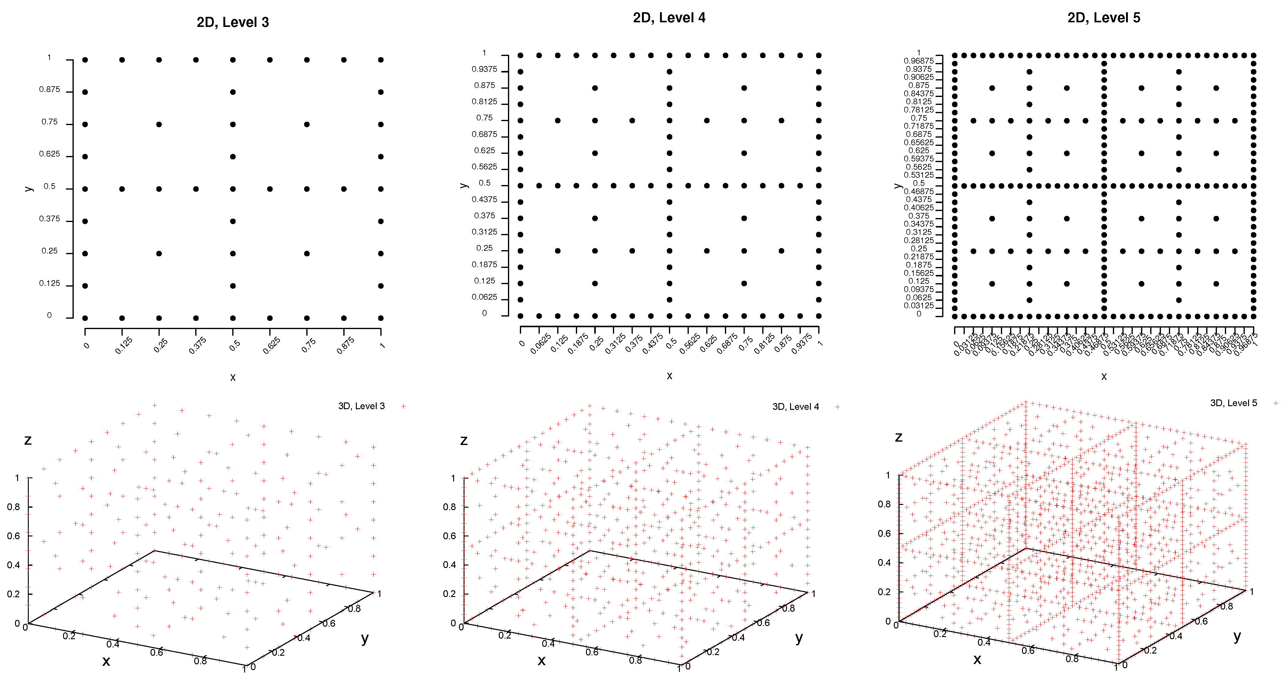
2.1. Interpolation on Sparse Grids

The interpolation on sparse grids is a highly efficient discretization method in the field of Finite Element Methodology (FEM). In contrast to full grids, sparse grids possess significantly less grid points, especially in high dimensional spaces. The computational effort decreases from O ( h - N ) to O ( h - 1 × ( log h - 1 ) N - 1 ) , where h is the mesh size of the full grid. In the meantime, the interpolation error increases from O ( h 2 ) to O ( h 2 × ( log h - 1 ) N - 1 ) only, with respect to the L -norm [28]. The interpolation is founded on a tensor product approach for high dimensions and a linear combination of basis functions, e.g., of hierarchical hat functions [29]. Thereby, the basis functions with small coefficients within the linear combination are left out, and the remaining basis functions correspond to points of a sparse grid. Here, the combination technique by [24] is used, an efficient methodology interpolating a function on regular subgrids. The combination of these subgrids results in a sparse grid. The most important application of interpolation on sparse grids is the solution of partial differential equations, cf. [30].

2.1.1. Idea of Sparse Grids

The main idea of sparse grids is to reduce the computational effort without obtaining an intolerable increase of the interpolation error. Especially in high dimensions, the reduction of computational effort becomes notable; Table 1 shows the number of grid points of full and sparse grids of different resolutions and dimensions. In the following, full and sparse grids are introduced with the aid of basis functions for piecewise-bilinear functions, i.e., for the two-dimensional case:
Table 1. Comparison of the number of grid points on full and sparse grids of different levels and dimensions. Especially for high levels and dimensions, the computational effort decreases significantly using sparse grids.
Level N = 1 N = 2 N = 3 N = 4
13 → 39 → 927 → 2781 → 81
25 → 525 → 21125 → 81625 → 393
39 → 981 → 49729 → 2256561 → 1329
417 → 17289 → 1134913 → 59383521 → 3921
101025 → 10251.05 × 10 6 92171.07 × 10 9 471031.1 × 10 12 1.78 × 10 5
Let Ω i , j be the equidistant rectangular grid on the unit square, Ω : = [ 0 , 1 ] 2 , with mesh sizes h i : = 2 - i in x- and h j : = 2 - j in the y-direction. The vector, : = ( i , j ) N 2 , is called level of the grid, Ω i , j , with one-norm | | 1 : = i + j . Moreover, let S i , j be the space of piecewise-bilinear functions on the grid, Ω i , j . For reasons of simplicity, only those piecewise-bilinear functions are considered here, which fulfill homogeneous Dirichlet boundary conditions in Ω i , j . The respective space is denoted by S i , j 0 . It can be expressed as a tensor product of subspaces T s , t , s = 1 , . . . , i , t = 1 , . . . , j , whose functions vanish on all grid points corresponding to S s - 1 , t 0 and S s , t - 1 0 :
S i , j 0 = s = 1 i t = 1 j T s , t
Uniquely determined piecewise-bilinear basis functions in T s , t with non-overlapping rectangular supports of size 1 / 2 s - 1 × 1 / 2 t - 1 are introduced; the so-called hierarchical basis [29]. Thereby, each grid point corresponds to a specific hierarchical basis function. It is situated in the center of the support. Moreover, each grid point belongs to a grid of a certain level, . The full grid results from the combination of these grids, and the direct sums of the hierarchical basis functions are the standard basis functions of the full grid.
Each function, u S i , j 0 , can be expressed by a linear combination of hierarchical basis functions:
u = s = 1 i t = 1 j u s , t , u s , t T s , t , s = 1 , . . . , i , t = 1 , . . . , j .
In [29], the inequality:
u s , t 4 - s - t - 1 | u |
was proven, where the seminorm, | u | , is given by:
| u | : = 4 u x 2 y 2
In order to obtain a sparse grid, only the functions whose coefficients are greater than or equal to a certain tolerance value are chosen. In [29], this tolerance value is set to 4 - ^ - 1 | u | , where ^ is the level of the sparse grid, which is defined in the following. All remaining basis functions are neglected, and a sparse grid space can be defined as follows:
Definition 1 (Sparse grid space) The space, S ^ ^ 0 , spanned by the subspaces, T i , j , with i + j = ^ + 1 , i.e.,
S ^ ^ 0 : = s = 1 ^ t = 1 ^ - s + 1 T s , t = s + t ^ + 1 T s , t
is called the sparse grid space. The grid resulting from the combination of the subgrids corresponding to the subspaces, T s , t , s + t ^ + 1 , is called the sparse grid and has the level, ^ .
The condition, | | 1 ^ + 1 , leads to a triangular scheme of subspaces, T i , j , which is depicted in Figure 4. Please note that k = 0 , k { 1 , 2 } , is feasible, but it must hold k { 1 , 2 } k < ^ . The transition to N-dimensional sparse grids of the level, ^ , is trivial: all subgrids of the level, , with | | 1 ^ + N - 1 k = 1 , . . . , N k < ^ have to be combined, where | | 1 = i = 1 N i .
Figure 5 shows some examples of sparse grids of the levels 3, 4 and 5 in 2D and 3D, which were produced with an algorithm combining sparse grids of a given level from the respective subgrids.
The coefficients corresponding to grid points of a grid with a high level do not contribute considerably to the interpolant. Hence, they can be neglected. However, a drawback of the sparse grid interpolation is the fact that this is only possible for functions that are sufficiently smooth. Because of inequality in Equation (6), the function that is interpolated must be at least four times continuously differentiable. Otherwise, the estimate cannot be made. As differentiability cannot be assumed in the present application, the combination technique developed by [24] is used here. A second problem concerning the computational effort is that sparse grids are still fully occupied at the boundary, cf. Figure 5. This problem can be handled using a transformation that sets the loss function to zero at the boundary. The methodology applied for SpaGrOW is described in the following.
Figure 4. Triangular scheme for the combination of a sparse grid of level 3 from two-dimensional subgrids meeting the condition, | | 1 3 + 2 - 1 = 4 k { 1 , 2 } k < 3 . If all eight subgrids are combined, a full grid of level 3 is obtained. If only the subgrids of levels (0,0), (1,0), (2,0), (3,0), (0,1), (0,2), (0,3), (1,1), (2,1), (1,2), (2,2), (3,1) and (1,3) are taken, i.e., if the small triangle consisting of three grids at the bottom right is left out, the corresponding sparse grid is obtained, cf. Figure 5 top left.
Entropy 15 03640 g004
Figure 5. Sparse grids of the levels 3, 4, and 5 in 2D and 3D.
Entropy 15 03640 g005

2.1.2. Combination Technique

The combination technique developed by [24] combines problems on regular grids of the level, , with different mesh sizes, 1 , . . . , N , to a sparse grid problem in a very efficient way. As this method has proven of value in practical applications and as it is also applicable to functions that are not necessarily smooth, it is taken as the sparse grid interpolation method for SpaGrOW.
As before, the two-dimensional case is considered first: Let u : R 2 R be an arbitrary function. Every function defined on a sparse grid can be linearly combined from their interpolants on the regular subgrids, Ω i , j , i + j { ^ , ^ + 1 } . If u i , j T i , j is considered, a combination function, u ^ c , can be defined as follows:
Definition 2 (Combination function (2D)). The combination function of solutions u i , j T i , j of FEM problems on regular two-dimensional grids of the level, ( i , j ) , i + j { ^ , ^ + 1 } , is given by:
u ^ c : = i + j = ^ + 1 u i , j - i + j = ^ u i , j
The error, u - u ^ c , is in O h ^ 2 log ( h ^ ) - 1 , cf. Section 3.3.1. Analogous to Definition 2, the following definition is given for the three-dimensional case:
Definition 3 (Combination function (3D)). The combination function of solutions u i , j , k T i , j , k of FEM problems on regular three-dimensional grids of the level, ( i , j , k ) , i + j + k { ^ , ^ + 1 , ^ + 2 } , is given by:
u ^ c : = i + j + k = ^ + 2 u i , j , k - 2 i + j + k = ^ + 1 u i , j , k + i + j + k = ^ u i , j , k
Via complete induction, this can directly be transferred to the N-dimensional case:
Definition 4 (Combination function (in general)). The combination function of solutions u T of FEM problems on regular N-dimensional grids of the level, ℓ, with | | 1 = ^ + N - 1 - i , i = 0 , . . . , N - 1 , is given by:
u ^ c : = i = 0 N - 1 ( - 1 ) i N - 1 i | | 1 = ^ + N - 1 - i u
Remark 5. Because of the condition, | | 1 = ^ + N - 1 - i , i = 0 , . . . , N - 1 , a multilinear interpolation on a full regular grid with mesh size 1 / 2 ^ and level ¯ = ( ^ ) can be executed as follows: All function values are computed on a sparse grid of the level, ( ^ , . . . , ^ ) N N . Because of the hierarchical structure of the sparse grid, all function values of the regular subgrids of the level, ℓ, with | | 1 ^ + N - 1 are known, i.e., all function values required for the interpolation, cf. Equation (11).

2.2. Smoothing Procedures

As already mentioned, the combination technique is applicable to functions that are not necessarily differentiable. However, an assumption of this method is the existence of an asymptotic error expansion for the discrete solution, cf. Section 3.3.1. Hence, the function to be interpolated should possess certain smoothness properties. At least, the statistical noise has to be filtered out as effectively as possible, and the quality of the continuity of the loss function should be high enough. As noise can be unfavorable for the combination technique, smoothing procedures have to be applied before the piecewise-linear interpolation is performed. In SpaGrOW, radial basis functions (RBFs) have turned out to be very suitable in order to approximate the loss function. In some cases, especially close to the minimum, a simple quadratic model is sufficient, as well. Additionally, the noise is filtered out via regularization procedures. In the approximation process, the respective nonlinear regression problem is not solved via least squares, but estimators with a lower variance. The regularization methods used in SpaGrOW are elastic nets and multi-adaptive regression splines. The applied smoothing and regularization algorithms are described in brief, and a theoretical selection is presented and discussed in the following. The final decision can only be made after a detailed practical evaluation, which is performed in Section 4.1.

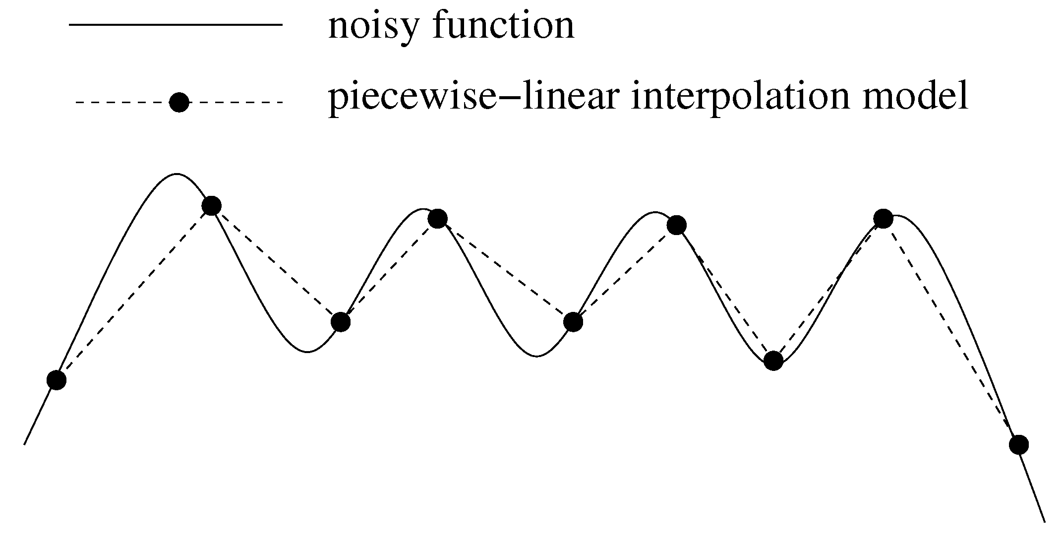
2.2.1. Effects of Statistical Noise on Piecewise-linear Interpolation

Suppose u is linear and noisy. Then, the piecewise-linear interpolation should reproduce the function exactly. However, statistical noise can lead to a staggered function, which is shown in Figure 6. As this is not desired, a preprocessing, which approximates the function to be interpolated and eliminates the noise, is indispensable.
Figure 6. Problematic in the case of piecewise-linear interpolation of a noisy function, the interpolation leads to a staggered function reproducing the noise.
Entropy 15 03640 g006
However, another problematic may appear whenever the sampled points used for the approximation are situated too close to each other: Figure 7 indicates that in this case, the trend of the function can be reproduced completely incorrectly. Therefore, SpaGrOW has to deal with this phenomenon, and the size of the trust region becomes too small has to be avoided.
Figure 7. Problematic in the case of the approximation of a noisy function, when the points are situated too close to each other, the function values cannot be differentiated anymore, and the trend of the function can be reproduced completely incorrectly by the smoothing procedure.
Entropy 15 03640 g007

2.2.2. Smoothing Functions

In the following, the approximation of high-dimensional functions with radial basis functions (RBFs) is presented shortly.
RBFs are an efficient and common method for interpolation and approximation tasks [31]. The word radial indicates that they are functions of the distance of two adjacent points. Hence, points which are situated on a hyperball with radius r around a reference point have the same function value. Here are some examples:
ϕ ( r ) = r ( linear )
ϕ ( r ) = exp - c r 2 , c R + ( Gaussian )
ϕ ( r ) = r 2 + c 2 , c R 0 ( multiquadric )
ϕ ( r ) = 1 r 2 + c 2 , c R 0 ( inverse multiquadric )
ϕ ( r ) = r 3 ( cubic )
ϕ ( r ) = r 2 log r ( thin plate splines )
A function, f : R N R , is approximated by:
f ( X ) i = 1 K β i h i X - X i
where X R N is an arbitrary test point and K m , where m N is the total number of points. The points, X i R N , i = 1 , . . . , K , are the K representative centers of the training set, on the basis of which the coefficients, β i R , i = 1 , . . . , K , are determined. The functions, h i H , i = 1 , . . . , K , are from the set of RBFs, H . The computation of the coefficients is realized by so-called RBF networks, cf. Figure 8, which are directed neuronal networks [32] and proceed from the input to the output neurons. They possess one layer of hidden neurons only, which corresponds to the determination of the coefficients. In the case of an approximation, it holds m K , and the following overdetermined linear equation system (LES) has to be solved:
H β = Y
where:
H = h 1 X 1 - X 1 h 2 X 1 - X 2 h K X 1 - X K h 1 X 2 - X 1 h 2 X 2 - X 2 h K X 2 - X K h 1 X m - X 1 h 2 X m - X 2 h K X m - X K R m × K
and:
Y = y 1 y 2 y m = f ( X 1 ) f ( X 2 ) f ( X m ) R m
The solution vector, β : = ( β 1 , . . . , β K ) T R K , can be computed e.g., by using least squares.
In order to select K representative centers out of the m training data in an efficient way, an unsupervised learning method is used, namely the automated classification (clustering) procedure, k-means [33]. The K centers are also the centroids of the data classes obtained by the clustering algorithm.
A drawback of RBFs is the high computational effort required for the collocation of the matrix, H, in Equation (19). For N = 5 , more than one thousand and for N = 6 , over 72 million RBF evaluations are necessary. Hence, RBFs should not be used for N > 4 .
For dimensions optimization problems, a simpler smoothing procedure is applied, whose complexity is only quadratic in the dimension. Instead of approximating the loss function itself, each of the physical target properties is approximated linearly, which results in a quadratic model of the loss function. This method is called linear property approximation (Lipra) and only requires the solution of an LES of the size N on a sparse grid. The loss function values can easily be obtained by inserting the approximated physical properties into the loss function. The complexity of the Lipra algorithm depends on the number of properties n and the dimension, N. It is O ( n N 2 ) .
Figure 8. Radial basis function (RBF) network: The network proceeds for a test point, X, from the input neurons, X j , j = 1 , . . . , N , (components of X), over a layer of hidden neurons containing the RBF evaluations, h i ( X - X i ) , i = 1 , . . . , K , with the coefficients, β i , i = 1 , . . . , K , to the output neuron, where the summation takes place. The result is the function value, f ( X ) .
Entropy 15 03640 g008

2.2.3. Regularization Algorithms

In order to avoid overfitting, the statistical noise the simulation data is affected with has to be eliminated. Therefore, the regression coefficients computed within the smoothing procedure may not be overestimated, so that not too much stress is laid on noisy data points. This can be achieved by a weighted regression, where a weighting factor is assigned to each data point that is small, whenever the noise on its function value is high, and vice versa. Another way is to constrain the coefficients in the optimization problem contained in the regression procedure. These so-called regularization algorithms do not solve the regression problem with the least square estimator, β LS , but with low-variance estimators. The former is given by:
β LS = arg min β | | Y - H β | | 2 2
and has the following drawbacks:
(1)
Due to its high variance, the probability of overfitting is always high.
(2)
The euclidean norm, | | β LS | | 2 , is, in general, high, as well.
(3)
There is no variable selection, i.e., none of the coefficients of β LS can be zero. Hence, correlated variables have always an influence within the model, even if they do not have any impact on the loss function.
(4)
If the dimension is greater than the number of data points, the least square method does not have a solution. However, due to K < < m , this is not important in the present case.
In order to counteract these drawbacks, the regression coefficients have to be shrinked or set to zero in some cases (variable selection). This has the effect that especially correlated variables and outliers only have low influence within the model. Moreover, the variance of the estimator is reduced, so that the probability of overfitting decreases. In SpaGrOW, this is realized by a Naive Elastic Net [34]:
β NEN = arg min β | | Y - H β | | 2 2 , where α | | β | | 2 2 + ( 1 - α ) | β | 1 t , α [ 0 , 1 ] , t > 0
It contains two additional model parameters, α [ 0 , 1 ] and t R > 0 , which can be determined, e.g., by a ten-fold cross-validation. A naive elastic net possesses a so-called grouping effect, i.e., correlated model variables have similar regression coefficients. A penalized formulation of Equation (21) is achieved by introducing Lagrangian multiplicators, λ 1 , λ 2 0 :
β NEN = arg min β L ( β , λ 1 , λ 2 ) , L ( β , λ 1 , λ 2 ) : = | | Y - H β | | 2 2 + λ 2 | | β | | 2 2 + λ 1 | β | 1
It holds α = λ 2 λ 1 + λ 2 . For α { 0 , 1 } , the two most famous methods in the field of biased regression are obtained: for α = 1 , it is the Ridge Regression [35], and for α = 0 , it is the Least Absolute Shrinkage and Selection Operator (LASSO) [36]. Both methods contain shrinkage, but only in the case of the LASSO, a variable selection is possible. For more details about Elastic Nets, Ridge Regression and the LASSO, cf. [34].
Another regularization method is based on the application of Multivariate Adaptive Regression Splines (MARS) [37]. The basis functions within this algorithm are products of so-called hinge functions of the order q N :
S q ( x ) = S q ( x - ν ) : = [ ± ( x - ν ) ] + q , q N
where ν is a node. “+" means that for negative arguments, the functions becomes zero. Two hinge functions with opposite sign belong together and are mirrored at their common node. Hence, they divide the input space into two disjoint subsets. By the recursive selection of p nodes, the input space is divided into p + 1 disjoint subsets. A single hinge function or a product of hinge functions, which lead to even more divisions, is assigned to each subspace. This models the interaction of the input variables. The approximation of a function, f : R N R , within the MARS algorithm is realized as follows:
f ( x ) i = 1 p ( β M ) i j = 1 s i S q ( x N ( i , j ) - ν i , j )
Thereby, the s i are the numbers of hinge functions considered in the partitioning, i { 1 , . . . , p } , ν i , j , i = 1 , . . . , p , j = 1 , . . . , s i are the nodes of the recursive division and N ( i , j ) is the dimension of the input vector, x, to which the division defined by the node ν i , j refers. In total, f is approximated by a regression spline and, in the case of q = 1 , by a piecewise-linear function. The lower probability of overfitting is reached by pruning the basis functions involved in the model. For more details about MARS, cf. [37]. A disadvantage of this regularization algorithm is the fact that it requires high computational effort for higher dimensions, due to the pruning procedure.
Please note that in the case of the Lipra algorithm, which is used for high-dimensional problems, no regularization procedure is applied, due to the high amount of computational effort.

2.2.4. Selection of Smoothing Procedures: Theoretical Considerations

The selection of the best smoothing procedure is made first from a theoretical perspective. A detailed practical evaluation is pointed out in Section 4.1. Theoretically, an approximation method can be selected, due to a reliable estimate of the approximation error within a domain, Ω R N . Such estimates exist for positive definite RBFs, cf. [38]. The Gaussian, the inverse multiquadric and so-called Wendland functions [39] are positive definite. The latter are RBFs with compact supports and are piecewise polynomial with a minimal degree dependent on differentiability and dimension.
An estimate of the approximation error can be realized via the introduction of Native Spaces [38]:
Definition 6 (Native Spaces). The Native Space, N ϕ ( Ω ) , for a given positive definite RBF, ϕ , within the domain, Ω, is given by:
N ϕ ( Ω ) : = { ϕ ( | | · - x | | ) , x Ω } ¯
where for f 1 = k = 1 n 1 α k ϕ ( | | · - x k | | ) N ϕ ( Ω ) and f 2 = j = 1 n 2 β j ϕ ( | | · - x j | | ) N ϕ ( Ω ) :
f 1 , f 2 ϕ ( Ω ) : = k = 1 n 1 j = 1 n 2 α k β j ϕ ( | | x k - x j | | )
Thereby, n 1 , n 2 N , α k , β j R , k = 1 , . . . , n 1 , j = 1 , . . . , n 2 , and x k , x j Ω , k = 1 , . . . , n 1 , j = 1 , . . . , n 2 .
The Hilbert space N ϕ ( Ω ) is the completing of the pre-Hilbert space, { ϕ ( | | · - x | | ) , x Ω } . As the approximation error depends on the size of the domain, Ω, the so-called fill distance is defined next:
Definition 7 (Fill distance). For a given discrete training set, X Ω , with training data, x j , j = 1 , . . . , m , m N , the fill distance, Δ Ω , X , is defined by:
Δ Ω , X : = sup x Ω min j = 1 , . . . , m | | x - x j | |
From Definitions 6 and 7, the following theorem for the estimation of the approximation error can be formulated:
Theorem 8 (Approximation error for positive definite RBFs). Let Ω , X , ϕ and f be defined as above. Let, furthermore, g be the approximating function for f N ϕ ( Ω ) , obtained by the positive definite RBF, ϕ . Then, the following estimate for the approximation error holds:
| | f - g | | L ( Ω ) h ( Δ Ω , X ) | | f | | N ϕ ( Ω )
where lim Δ Ω , X 0 h ( Δ Ω , X ) = 0 .
Proof. [38]          ☐
This theorem is very important for the convergency of SpaGrOW, cf. Section 3.3.2. However, for SpaGrOW, another condition, lim Δ Ω , X 0 h ( Δ Ω , X ) = 0 , has to be fulfilled. The following definition introduces the term stability of an approximation in the sense of SpaGrOW:
Definition 9 (Stable approximation). Let Ω and X be defined as above. Let be f H , where H is a Hilbert space of functions on Ω with the scalar product, · , · H , and norm | | f | | H = f , f H for f H . An approximation within the domain, Ω, by a function, g P , where P is a pre-Hilbert space with the same scalar product and P ¯ = H , is called stable, if:
| | f - g | | H κ h ( Δ Ω , X )
where κ > 0 , lim Δ Ω , X 0 h ( Δ Ω , X ) = 0 and lim Δ Ω , X 0 h ( Δ Ω , X ) Δ Ω , X = 0 .
The second important condition for the convergency of SpaGrOW is lim Δ Ω , X 0 h ( Δ Ω , X ) Δ Ω , X = 0 . The following corollary ascertains the stability of an approximation based on a Gaussian RBF:
Corollary 10 (Stability of an approximation based on a Gaussian RBF). Let Ω , X and f be defined as in Theorem 8. Let, furthermore, ϕ ( | | · - x | | ) = exp - c | | · - x | | 2 for x Ω and c R + a Gaussian RBF. Then, the approximation of f by g ( x ) : = k = 1 ν α k ϕ ( | | x k - x | | ) , ν N , α k R , x k Ω , k = 1 , . . . , ν , is stable.
Proof. For a Gaussian RBF, the following estimation holds (cf. [38]):
| | f - g | | L ( Ω ) exp - d log ( Δ Ω , X ) Δ Ω , X | | f | | N ϕ ( Ω )
where d > 0 is a constant. With h ( Δ Ω , X ) : = exp - d log ( Δ Ω , X ) Δ Ω , X , it holds lim Δ Ω , X 0 h ( Δ Ω , X ) = 0 and lim Δ Ω , X 0 h ( Δ Ω , X ) Δ Ω , X = 0 . With κ : = | | f | | N ϕ ( Ω ) and the fact that N ϕ ( Ω ) is a Hilbert space and g an element of the pre-Hilbert space, { ϕ ( | | · - x | | ) , x Ω } , with { ϕ ( | | · - x | | ) , x Ω } ¯ = N ϕ ( Ω ) , it follows that the approximation based on a Gaussian RBF is stable with respect to Definition 9.      ☐
Because of Corollary 10, the Gaussian RBF is selected for SpaGrOW for theoretical reasons. However, such estimates exist for other positive RBFs, as well. The final selection of the Gaussian RBF is made after a detailed practical evaluation, as mentioned above.

3. The SpaGrOW Algorithm

3.1. Ingredients of the Algorithm

Within SpaGrOW, the minimization of the interpolation model on a full grid is performed discretely. The corresponding complexity is O ( n + 1 ) 2 N , where n + 1 ( n N ) is the number of points of the full grid in one dimension. The first question arising is whether the algorithm should be applied locally or globally. Globally, this means that the smoothing procedure and the sparse grid interpolation are performed on the complete feasible domain for the force field parameters. However, it results that a local consideration is the better way, i.e., the combination with the Trust Region approach is highly important. This makes SpaGrOW an iterative local optimization method. The algorithm is described in detail in the following.

3.1.1. Local and Global Consideration

The combination technique delivers a piecewise-multilinear function, q : R N R , which either interpolates the loss function, F, itself or an approximating function, G, from a sparse grid of the level, ^ N , on a full grid, G ¯ N , with the level, ¯ = ( ^ , . . . , ^ ) N N . The total error resulting from the approximation and interpolation error can be measured via the L 2 - or L -distance between F and the interpolation model, q, on the unit square, Ω : = [ 0 , 1 ] N :
| | e | | L 2 , [ 0 , 1 ] N : = | | F - q | | L 2 , [ 0 , 1 ] N = [ 0 , 1 ] N F ( x ) - q ( x ) 2 d x 1 2
| | e | | L , [ 0 , 1 ] N : = | | F - q | | L , [ 0 , 1 ] N = max x [ 0 , 1 ] N | F ( x ) - q ( x ) |
If the function values, F ( x ) , are known for x G ¯ N , the error terms in Equations (31) and (32) can be approximated numerically.
The total error is important for the assessment of whether SpaGrOW can be applied globally or not. Hence, it has to be determined on a full grid for the local and the global variant. Moreover, the convergency behavior of SpaGrOW has to be analyzed. There are some arguments for a local consideration: Following the heuristics indicated in Section 2.2, it is indispensable to perform a smoothing procedure before interpolating. In the global case, this smoothing procedure would be executed on a sparse grid discretizing the complete feasible domain. As the loss function can be arbitrarily complex and jagged, it should be nearly impossible to reproduce them in an accurate way within a huge domain with only a small number of data points. Furthermore, the discretization error would be too high within a huge domain for the determination of the global minimum. However, it would be possible to apply the algorithm globally first and to make local refinements afterwards, but an inaccurate approximation of the loss function can lead far away from the minimum. Hence, a local consideration should be preferred, and SpaGrOW should be a local iterative procedure, like the gradient-based methods applied for the present task.
In order to verify these heuristic considerations, a practical analysis was performed, where the loss function was replaced by the simple two-dimensional function, H ( x 1 , x 2 ) = - exp - ( x 1 - 2 ) 2 - ( x 2 + 1 ) 2 . The global minimum is situated at x 1 * , x 2 * = ( 2 , - 1 ) , with corresponding function value, H ( 2 , - 1 ) = - 1 . Artificial statistical uncertainties, i.e., uniformly distributed random numbers from the interval, [ - 0 . 03 H ( x 1 , x 2 ) , + 0 . 03 H ( x 1 , x 2 ) ] , were added on the function values, H ( x 1 , x 2 ) . For reasons of brevity, the analysis is not reported here. The results were the following:
  • Comparison of the total errors:
    In the global consideration, the total errors were significantly higher than in the local consideration with respect to both the L 2 - and the L -norm.
    The smoothing error is considerably higher in the global case than in the local one, i.e., the function cannot be reproduced accurately. This was also the case when the function was not affected with statistical noise.
  • Convergency analysis:
    Without artificial uncertainties, the global variant of SpaGrOW only led to the minimum when the minimum was a grid point. Otherwise, the minimum could only be determined within the accuracy of the discretization.
    With artificial uncertainties, both discretization and approximation error had a negative effect on the convergency. The resulting approximated minimum was far away from the real one.
To summarize, a local consideration is preferred to a global one.

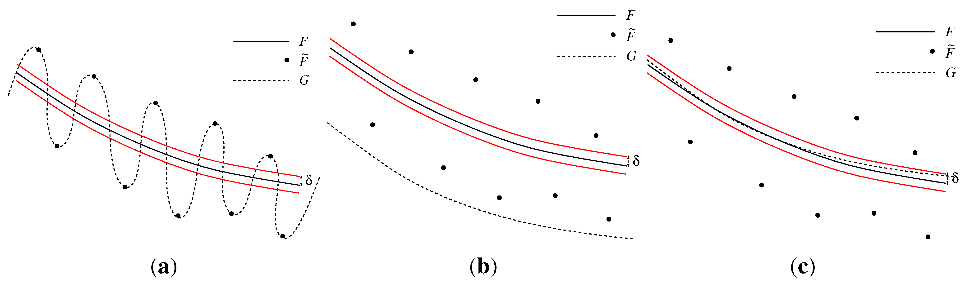
3.1.2. Combination with the Trust Region Approach

For each iteration, a compact neighborhood, where the minimization problem is solved discretely, is determined. In most cases, the minimum is situated at the boundary of the compact domain. If certain assumptions are fulfilled, this boundary minimum becomes the new iteration and the center of a new compact neighborhood.
Following the idea of Trust Region methods [25,26], the compact neighborhood is a trust region of the size, Δ k > 0 . Due to the sparse grid interpolation, it is not a ball, B Δ k ( x k ) , but a hyperdice, W k , of the form:
W k : = i = 1 N x i k - Δ k , x i k + Δ k
where x k is the kth iteration of SpaGrOW. On the one hand, the size, Δ k , has to be small enough, so that W k is situated within the feasible domain of the force field parameters and the interpolation model is consistent with the original loss function, F, as already discussed in Section 3.1.1. On the other hand, Δ k has to be large enough, so that the method converges as fast as possible to the global minimum within the feasible domain. Hence, the division of the domain into non-disjoint hyperdices should not be too fine.
The quality of the model, q, is estimated using the following ratio:
r k : = F ( x k ) - F ( x * ) q ( x k ) - q ( x * ) = F ( x k ) - F ( x * ) G ( x k ) - q ( x * )
where x * is the discrete minimum on a full grid within the hyperdice, W k . As x k is a point of the sparse grid and the model, q, interpolates the approximating function, G, from the sparse grid on the full grid, it holds q ( x k ) = G ( x k ) .
In practice, two thresholds, 0 < η 1 < η 2 , and size parameters, 0 < γ 1 < 1 < γ 2 , are introduced, and the following three cases are considered:
  • η 2 > r k η 1 —in this case, the model is consistent with F, and the minimum, x * , is taken as a new iteration: x k + 1 : = x * .
  • r k η 2 > η 1 —then, x * is taken as a new iteration, as well, and at the same time, the trust region is increased in order to accelerate the convergency: Δ k + 1 : = γ 2 Δ k .
  • r k < η 1 —in this case, the model is not consistent with F, and a better model has to be determined by decreasing the trust region: Δ k + 1 : = γ 1 Δ k .
As for the Trust Region methods, a minimal Δ min > 0 is defined a priori. The algorithm is stopped as soon as k : Δ k < Δ min .

3.1.3. Treatment of Boundary Points

After the application of a transformation, ξ : W k [ 0 , 1 ] N , into the unit hyperdice, cf. Section 3.2.1, the loss function values are set to zero at its boundary by an appropriate modification. The reason of the realization of homogeneous Dirichlet boundary conditions is the fact that also sparse grids are fully occupied at their boundaries. In order to save a magnitude of simulations, the original loss function, F, is multiplied with a product of sine functions, i.e., the modified function:
F ¯ : [ 0 , 1 ] N R 0 +
y i = 1 N sin π y i F ( y )
where y = ξ ( x ) with x W k is considered instead of F. Hence, the smoothing and interpolation procedures are applied for F ¯ ξ : W k R 0 + . Due to Equation (35), it holds F ¯ | [ 0 , 1 ] N = 0 . However, as F and not F ¯ has to be minimized and as F and F ¯ do not have the same minimum, the back-transformation:
F ( x ) = F ( ξ - 1 ( y ) ) = F ¯ ( y ) i = 1 N sin π y i
has to be applied before the discrete minimization is performed. Hence, the minimum of F ξ - 1 has to be determined, which is not possible at the boundary of W k . As the minimum is expected to be situated at the boundary, only the grid:
G ˜ ¯ N : = G ¯ N \ G ¯ N
is considered for the minimization. This grid does not contain any boundary point of the original grid. However, this reduces the size of the trust region, but the loss in convergency speed is negligible, due to the number of simulations to be saved; for N = 4 and ^ = 2 , only nine instead of 393 simulations (cf. Table 1) per iteration are required.

3.2. The Full Algorithm

3.2.1. Structure

The algorithm of SpaGrOW, i.e., the inner iteration of the optimization procedure shown in Figure 1, is visualized in Figure 9 and has the following structure:
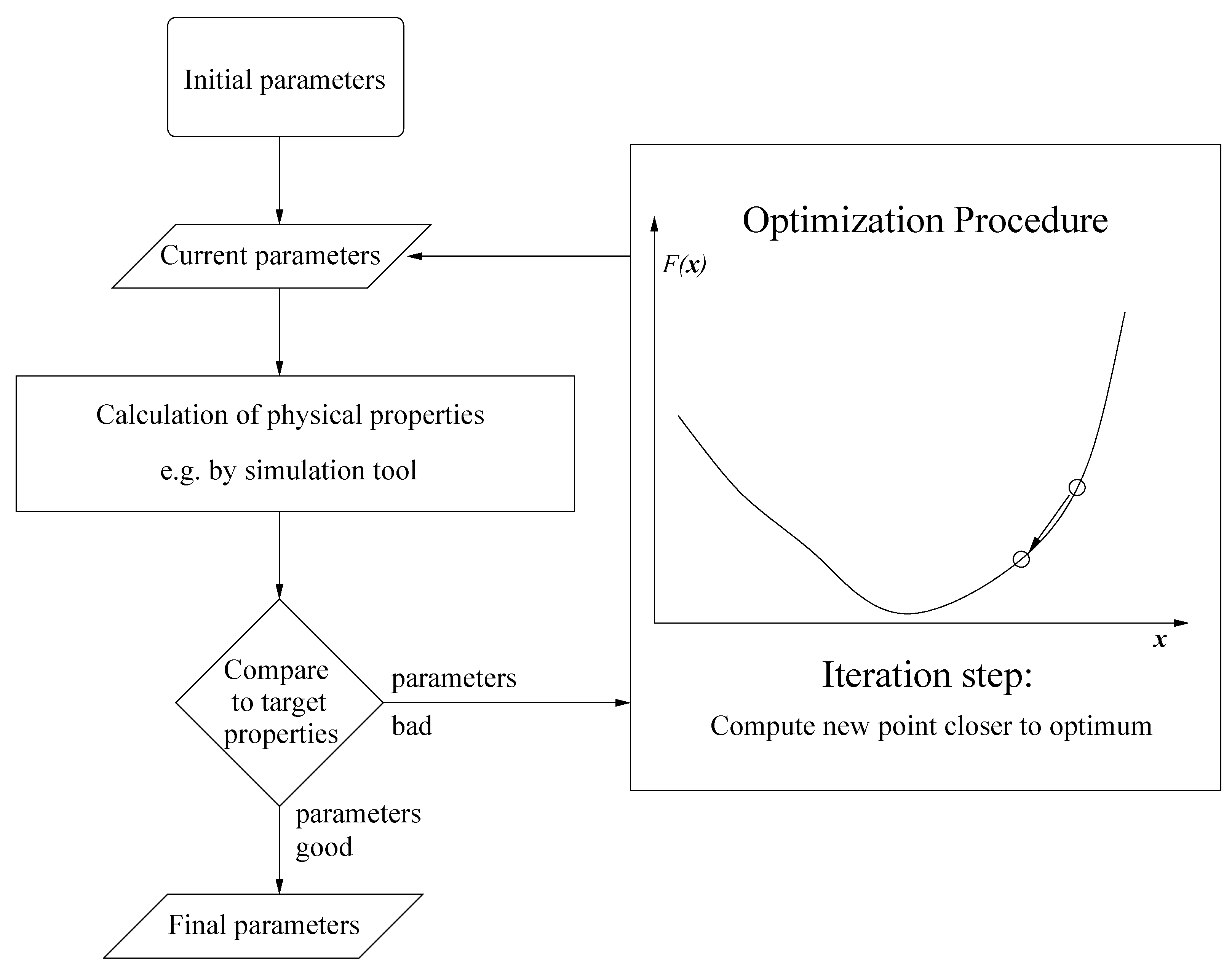
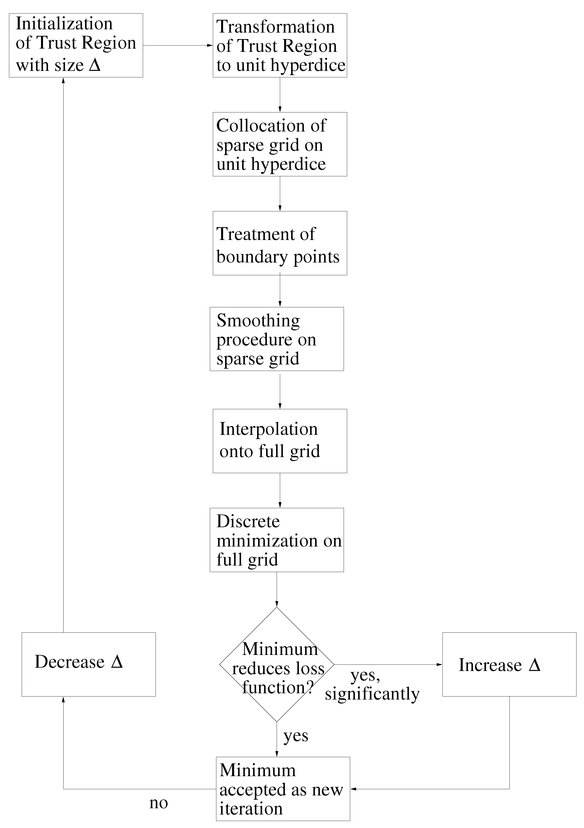
  • Initialization: Choose an initial vector, x 0 , and an initial step length, D 0 > 0 , so that:
    i = 1 , . . . , N c i 0 x i 0 C i 0 , Δ 0 < C i 0 - x i 0 , Δ 0 < x i 0 - c i 0
    Thereby, [ c i 0 , C i 0 ] is the feasible interval for the ith force field parameter. The maximal step length possible, Δ max , is computed at the beginning, and Δ 0 , as well as a minimal step length, Δ min , are set in relation to it. Please note that on the one hand, Δ 0 must not be too small, due to the noise, and that, on the other hand, it must not be too large, so that the problematic described in Section 3.1.1. is not faced.
    Let k : = 0 .
    Figure 9. Overview of the SpaGrOW algorithm, i.e., the inner iteration of the optimization procedure visualized in Figure 1. The Trust Region size, Δ, is increased or decreased, depending on the quality of the approximation model on the sparse grid.
    Figure 9. Overview of the SpaGrOW algorithm, i.e., the inner iteration of the optimization procedure visualized in Figure 1. The Trust Region size, Δ, is increased or decreased, depending on the quality of the approximation model on the sparse grid.
    Entropy 15 03640 g009
  • Transformation: Via the transformation:
    ξ : W k [ 0 , 1 ] N x x - min i = 1 , . . . , N x i k · e max i = 1 , . . . , N x i k · e - min i = 1 , . . . , N x i k · e = 1 2 Δ k x - x k + Δ k · e
    the initial vector, x 0 , is mapped from the hyperdice of the size, Δ 0 , into the unit hyperdice. Thereby, e = ( 1 , . . . , 1 ) T R N and x i k , i = 1 , . . . , N are the components of the vector, x k .
    Please note that only the back-transformation obtained by the inverse function:
    ξ - 1 : [ 0 , 1 ] N W k y 2 Δ k y + x k - Δ k · e
    is important, because, first, a sparse grid is simply collocated in [ 0 , 1 ] N . Then, the grid points are back-transformed into the force field parameter space via ξ - 1 , so that molecular simulations can be executed.
  • Sparse grid: A sparse grid, G ^ ^ N , is determined within [ 0 , 1 ] N = ξ W k . Note that the transformation, ξ, has not to be applied explicitly. As the combination technique is used, the grid points of the sparse grid are determined hierarchically from the required subgrids, cf. Equation (11). Let y , j be a point of the subgrids of the level, = ( 1 , . . . , N ) , and position, j = ( j 1 , . . . , j N ) , which is, at the same time, a non-boundary point of the sparse grid. For each of these points, the loss function value, F ( y , j ) , is computed.
  • Boundary: By multiplying F with a sine term:
    F ¯ : [ 0 , 1 ] N R 0 +
    y i = 1 N sin π y i F ( y )
    homogeneous Dirichlet boundary conditions are realized in order to reduce the computational effort significantly. The function, F ¯ , is applied to each point, y , j , of the sparse grid.
  • Smoothing: As the function to be minimized is affected with statistical noise, the function, F ¯ , is smoothed and regularized by the methods indicated in Section 2.2.2. Hence, for each point, y , j , of the sparse grid, a value, G ( y , j ) , of the approximating function is obtained.
  • Interpolation: The function, G, is interpolated from the sparse grid, G ^ ^ N , on the full grid, G ¯ N , by the combination technique. Hence, an interpolation model, q ¯ , is obtained for each point, y G ¯ N .
    As the smoothing and interpolation procedures have been executed for F ¯ , the following division has to be applied for each non-boundary point of the full grid:
    y G ˜ ¯ N q ( y ) = q ¯ ( y ) i = 1 N sin π y i
    The interpolation model, q, is only valid for all y G ˜ ¯ N .
  • Discrete minimization: Determine:
    y * : = arg min y G ˜ ¯ N q ( y )
  • Iteration step x k x k + 1 : The ratio:
    r k : = F ( y k ) - F ( y * ) q ( y k ) - q ( y * ) = F ( y k ) - F ( y * ) G ( y k ) - q ( y * ) , y k = ξ ( x k )
    is determined, and the following three cases are differentiated:
    r k η 1 x k + 1 : = ξ - 1 ( y * ) Δ k + 1 : = Δ k .
    r k η 2 > η 1 x k + 1 : = ξ - 1 ( y * ) Δ k + 1 : = γ 2 Δ k
    r k < η 1 x k + 1 : = x k Δ k + 1 : = γ 1 Δ k .
    Thereby, η 2 > η 1 > 0 and γ 2 > 1 > γ 1 > 0 are global parameters.
    Let k : = k + 1 , and go to step 2.
  • Stopping criteria: The general stopping criterion is:
    F ( x * ) τ
    where τ > 0 . However, an additional criterion is that the minimum is situated within the hyperdice and not at its boundary. In total, the following three stopping criteria are considered:
    (i)
    F ( x * ) τ ξ ( x * ) U 0 U 1
    (ii)
    F ( x * ) τ ξ ( x * ) U 0 U 1 Δ * < Δ min
    (iii)
    k N : r k < η 1 Δ k < Δ min .
    Thereby:
    U 0 : = { y [ 0 , 1 ] N | i 1 , . . . , N : y i { 0 , 1 } } , U 1 : = { y [ 0 , 1 ] N | i 1 , . . . , N : y i { 2 - ^ , 1 - 2 - ^ } }
    Moreover, Δ * : = Δ k , where x * = x k .
    If the stopping criteria, (i) and (ii), are fulfilled, then SpaGrOW has converged successfully. Due to ξ ( x * ) U 1 , it is excluded, as well, that the minimum is situated at the boundary of the grid, where the interpolation model, q, is valid. Stopping criterion (ii) contains the additional condition, Δ * < Δ min , excluding that improvements can be achieved by local refinements. Hence, this is the ideal stopping criterion.
    Stopping criterion (iii) means that SpaGrOW has not led to success, i.e., even by decreasing the trust region, no accurate model, q, can be found. In particular, this is the case when the assumptions for the application of the combination technique are not fulfilled, which may be caused by an inaccurate smoothing procedure, wherein the noise has not been filtered out in a sufficient way.

3.2.2. Complexity

In the following, the complexity of SpaGrOW is discussed. The present section is organized like Section 3.2.1., but here, SpaGrOW is discussed with respect to complexity:
  • Initialization: The effort is only caused by the allocation of the initial variables, like the initial force field parameters, their upper and lower bounds, as well as the maximal, initial and minimal step length.
  • Transformation: The transformation is performed in an imaginary way only. The sparse grid is constructed directly in step 3. Only the execution of the back-transformation, ξ - 1 , requires a small computational effort.
  • Sparse grid: The complexity to obtain a sparse grid of the level, ^ , is O 2 ^ · ^ N - 1 , which is still exponential in the dimension, but especially in the case of higher dimensions, it is significantly lower than for a full grid of the same level. The computational effort does not only concern the number of grid points to be computed, but in the first instance, the number of loss function evaluations, i.e., simulations.
  • Boundary: Setting the loss function values to zero at the boundary of the sparse grid does not mean any computational effort. For all other grid points, 2 N + 1 ( O ( N ) ) multiplications have to be performed, cf. Equation (35). Furthermore, there are N sine evaluations. The number of boundary points of an N-dimensional sparse grid of the level, ^ , is O N 2 N - 1 2 ^ . Thereby, N 2 N - 1 is the number of edges of an N-dimensional hyperdice. Hence, the number of simulations to be executed is reduced to:
    O 2 ^ ^ N - 1 - N 2 N - 1
    This number multiplied by 2 N + 1 is the number of required multiplications and multiplied by N, the number of sine evaluations required. The reduction of molecular simulations is achieved at the expense of
    O N 2 ^ ^ N - 1 - N 2 N - 1
    multiplications and sine evaluations, a computational effort that can be neglected, if the high amount of computation time for a simulation is opposed.
  • Smoothing: In the case of most approximation methods, a multivariate linear regression has to be performed with complexity O ( m M 2 + M 3 ) , where m is the number of data points and M, the number of basis functions (e.g., M = K for RBFs). However, this complexity can often be reduced to O ( m M 2 + M 2 ) or, even, to O ( 1 ) by smart numerical methods, e.g., by a Cholesky factorization, in the case of positive definiteness. In contrast to simulations, the computational effort required for a smoothing procedure is negligible, as well. However, one has to consider that m and M must be large enough, on the one hand, in order to achieve an approximation as accurate as possible, and also small enough, on the other hand, in order to keep the computational effort low and to avoid overfitting. Additional effort appears due to the selection of centroids by the k-means algorithm, whose convergency speed always depends on the random choice of the initial centroids. The evaluation of the model function is done by a summation of the centroids only.
    Furthermore, the regularization methods require some amount of computational effort, in particular, due to the application of Newton-Lagrange algorithms for the constrained optimization. Please note that most of them have been parameterized, as well, e.g., by cross validation.
  • Interpolation: In the multilinear interpolation, all adjacent points have to be considered for each grid point. Hence, the interpolation is in O ( 2 N + 1 ) · 2 ^ · ^ N - 1 .
    After the multilinear interpolation, a division by a sine term has to be executed for each point situated inside the unit hyperdice. As the sine term has already been calculated for each point of the sparse grid, only:
    O ( 2 N + 1 ) ( 2 ^ - 1 ) N - 2 ^ ^ N - 1
    multiplications and:
    O N ( 2 ^ - 1 ) N - 2 ^ ^ N - 1
    sine evaluations have to be performed. The number of required divisions is equal to ( 2 ^ - 1 ) N . Please note that the divisions have to be performed for each inner point of the sparse grid, as well, because only the approximating function, G, coincides with the interpolation model, but not F ¯ .
  • Discrete minimization For the minimization of q, a maximal function value of 10 6 is supposed. For each point on the full grid, a comparison has to be performed, in total, ( 2 ^ - 1 ) N comparisons.
  • Iteration step: Only a few small operations are necessary in order to perform an iteration step, i.e., simple subtractions, divisions, multiplications and comparisons.
  • Stopping criteria: Only comparisons have to be performed in order to check the stopping criteria. The decision whether a vector is situated in U 0 U 1 or not is made by comparing the components of y with the values zero, one, h and 1 - h . If one component coincides with one of these four values, the procedure is stopped, and y U 0 U 1 is observed.

3.3. Convergency

In the following, some convergency aspects the SpaGrOW algorithm are considered. In [40], it was proven that the algorithm converges under certain assumptions. Thereby, both smooth and noisy objective functions were considered. In the smooth case, the interpolation error is relevant, and in the noisy case, the approximation error with respect to the original function, i.e., the function without noise, has to be taken into account. Moreover, it is examined to what extent SpaGrOW manages with less simulations than gradient-based methods. In the case of the latter, simulations have to be performed for the gradient components, the entries of the Hessian matrix and the Armijo steps. In the case of SpaGrOW, they have to be executed for the sparse grid points and the Trust Region steps. The steepest descent algorithm and the conjugate gradient methods required significantly less simulations for the gradient than SpaGrOW for the sparse grid: for N = 4 , four simulations are required for the gradient and nine for a sparse grid of the level 2. As for the step length control, it can be observed that both gradient-based methods and SpaGrOW mostly need one Armijo or, respectively, one Trust Region step at the beginning of the optimization, but many more close to the minimum. The reason for the reduction of computational effort in the case of SpaGrOW lies in the lower number of iterations, not in the lower number of function evaluations per iteration. The advantage is that the step length is determined before, so that, especially at the beginning of the optimization, large steps can be realized. For smooth functions, the combination technique delivers small interpolation errors in most cases, also when the trust region is quite large, but always a descent direction, mostly leading to the boundary of the actual trust region.
Close to the minimum, both approaches have the drawback that after a high number of step length control iterations, i.e., after a large computational effort, only marginal improvements in the loss function values are observed. However, due to the statistical noise, the minimum can never be predicted exactly. At some point, the minimization has to be stopped, and the actual result has to be evaluated. However SpaGrOW is capable of searching for a smaller loss function value in more than one direction, due to the grid approach. Furthermore, its modeling approach increases the probability to get close to the minimum than gradient-based methods, as motivated in Section 1.
As the interpolation and smoothing errors are essential for the convergency of SpaGrOW, they are introduced and discussed in the following.

3.3.1. Interpolation Error

Under certain assumptions [24], the interpolation error for a sparse grid of the level, ^ , is of the order O h ^ 2 log ( h ^ ) - 1 ^ - 1 . First, the two-dimensional case is considered again. If the difference u - u i , j , where u i , j T i , j , i + j { ^ , ^ + 1 } , meets point-wise an asymptotic error expansion, i.e.,
u - u i , j = C 1 ( h i ) h i 2 + C 2 ( h j ) h j 2 + D ( h i , h j ) h i 2 h j 2
where i | C 1 ( h i ) | κ , j | C 2 ( h j ) | κ and i , j | D ( h i , h j ) | κ , κ > 0 , then the interpolation error can be estimated as follows:
| u - u ^ ^ c | 1 + 5 4 log h ^ - 1 κ h ^ 2 = O h ^ 2 log ( h ^ ) - 1
For the N-dimensional case, an analogous asymptotic error expansion delivers the following formula:
| u - u ^ ^ c | l = 0 N - 1 χ l log h ^ - 1 l κ h ^ 2 = O h ^ 2 log ( h ^ ) - 1 ^ - 1
Thereby, u S ¯ 0 , ¯ = ( ^ , . . . , ^ ) N N and χ l N , l = 0 , . . . , ^ - 1 .
Please note that in order to guarantee the existence of such an asymptotic error expansion, the exact solution, u, must fulfill certain continuity and smoothness conditions. As u is supposed to reproduce F exactly on the sparse grid and as accurately as possible between the sparse grid points, these assumptions have to be transferred to F. This motivates again the need for a smoothing procedure in the case of statistical noise. In most cases, the existence of an asymptotic error expansion cannot be proven a priori. However, the combination technique was shown to deliver very good results in practice [24].
The interpolation error can be estimated above as follows:
Theorem 11 (Estimate for the interpolation error). Let Δ > 0 be the size of the hyperdice, W Δ ( x ) , with center x R N , where a sparse grid of the level, ^ , is defined. Let the approximated function, G : R N R 0 + , be given on the sparse grid and interpolated by the model function, q : B Δ ( 0 ) R , on a full grid of the level, : = ( ^ , . . . , ^ ) N N , using the combination method. Then, for the interpolation error, ε = | u - u ^ ^ c | , in Inequality (53), it holds for u : = G and u ^ ^ c : = q :
y W Δ ( x ) | ε ( y ) | κ ε ( ^ ) f ^ ε ( Δ )
where κ ε : N R + and f ^ ε : R + R + with lim ^ κ ε ( ^ ) = 0 and lim Δ 0 f ^ ε ( Δ ) = 0 . The function, f ^ ε , is continuous. Moreover, f ˜ ^ ε : = f ^ ε Δ : R + R + is continuous, as well, with lim Δ 0 f ˜ ^ ε ( Δ ) = 0 .
Proof. Let y W Δ ( x ) be an arbitrary point in the hyperdice. It holds h ^ = 2 1 - ^ Δ . Following Inequality (53), there exist constants χ l > 0 , l = 0 , . . . , N - 1 and a κ > 0 , so that:
| ε ( y ) | l = 0 N - 1 χ l log 2 ^ - 1 Δ - 1 l κ 2 2 - 2 ^ Δ 2
= l = 0 N - 1 χ l ^ - 1 - log Δ l κ 2 2 - 2 ^ Δ 2
N · max l = 0 N - 1 χ l · κ 2 2 - 2 ^ : = κ ε ( ^ ) · max l = 0 N - 1 ^ - 1 - log Δ l · Δ 2 : = f ^ ε ( Δ )
= κ ε ( ^ ) f ^ ε ( Δ )
It holds lim ^ κ ε ( ^ ) = 0 , and also, because of l’Hospital’s rule, lim Δ 0 f ^ ε ( Δ ) = 0 . Due to f ˜ ^ ε ( Δ ) = max l = 0 N - 1 ^ - 1 - log Δ l · Δ , it follows also from l’Hospital’s rule that lim Δ 0 f ˜ ^ ε ( Δ ) = 0 .           ☐

3.3.2. Smoothing Error

Let | | · | | be one of the two norms, | | · | | L 2 or | | · | | L . The smoothing error, μ, is the error with respect to | | · | | between the original function, F = F ˜ - Δ F , without noise and the approximating function, G. Thereby, F ˜ is the noisy function. It holds:
μ : = | | F - G | | = | | ( F + Δ F ) - G - Δ F | | = | | F ˜ - G - Δ F | | | ϑ | + | | Δ F | |
where ϑ denotes the training error. If Ω is a trust region, then define
x Ω ϑ ( x ) : = F ˜ ( x ) - G ( x ) . In the ideal case, ϑ ( x ) = Δ F x , it holds μ ( x ) = 0 . Otherwise, for 0 < δ < < | Δ F x | , the following inequation must hold:
| μ ( x ) | = | Δ F x - ϑ ( x ) | δ
This means that the training error, ϑ, must not be too small. Figure 10a shows an overfitted model, G, which reproduces exactly the oscillations produced by the noise. In this case, ϑ = 0 , but | μ ( x ) | = | Δ F x | > > δ for certain x Ω . On the other hand, the training error must not be too high. In Figure 10b, it holds x Ω | μ ( x ) | | Δ F x | > > δ . Only Figure 10c depicts a feasible case; here, the training error is in the same order as the noise, and it holds | μ | δ .
Figure 10. Approximation models with different training errors, ϑ, where the function, G, approximates the noisy function, F ˜ = F + Δ F , overfitted model with ϑ = 0 (a); model, where ϑ is too high (b); and feasible model with | Δ F - ϑ | δ (c). In the ideal case, it holds ϑ ( x ) = Δ F x .
Entropy 15 03640 g010
In order to keep the smoothing error low enough, a smoothing procedure has to be applied, which filters out the noise and reproduces the loss function, at least on the sparse grid, as exactly as possible. As a smoothing procedure can only be evaluated on a sparse grid, due to the high amount of computation time for molecular simulations, the condition, | μ | δ , is considered only on the sparse grid. It does not matter if G has oscillations between the sparse grid points, because the piecewise-multilinear sparse grid interpolation is not capable of modeling them anyway.
The following theorem is essential for the convergency proof of SpaGrOW and gives an estimate for the smoothing error in the case of positive definite RBFs:
Theorem 12 (Estimate for the smoothing error). Let Δ > 0 be the size of the hyperdice, W Δ ( x ) , with the center, x R N , in which a sparse grid of the level, ^ , is constructed. Let the loss function, F : R N R 0 + , be given on the sparse grid and approximated by the function, G : R N R . Suppose that the approximation be stable. Then, the smoothing error μ from Equation (56) can be estimated as follows:
κ μ > 0 : y W Δ ( x ) | μ ( y ) | κ μ f μ ( Δ )
where f μ : R + R + is continuous with lim Δ 0 f μ ( Δ ) = 0 . Furthermore, f ˜ ( μ ) : = f μ Δ : R + R + is continuous, as well, with lim Δ 0 f ˜ μ ( Δ ) = 0 .
Proof. Due to the stability of the smoothness, Inequality (29) holds, where Ω = W Δ ( x ) and X is the sparse grid. The fill distance on the sparse grid and Δ only differ by a constant, ω > 0 , i.e., Δ Ω , X = ω Δ . For κ μ : = κ and f μ ( Δ ) : = h ( ω Δ ) = h ( Δ Ω , X ) , the estimate for the smoothing error in Equation (58) follows directly.
Remark 13. Following Corollary 10, estimate Equation (58) is given in the case of a smoothing procedure based on Gaussian RBFs.
Remark 14. For Theorem 12 and the full convergency proof, it is irrelevant whether the original function, F : R N R 0 + , or the transformed function, F ¯ : [ 0 , 1 ] N R 0 + , is approximated by G : R N R . The function to be smoothed only has to be continuous within the trust region. Please note that in the case of F ¯ , the function, G, can have negative values, as F ¯ is equal to zero at the boundary of the trust region. For the original function, G ( x ) 0 can be assumed, due to Theorem 12, when Δ is small enough. For F ¯ , this can be assumed, as well. Otherwise, consider a translation that does not have any impact on either the approximation or the minimization.
The convergency proof executed for SpaGrOW was related to a general convergency proof for derivative-free Trust Region methods [41]. However, the Trust Region method used in that paper is based on an interpolation with Newtonian fundamental polynomials. Hence, the partial proofs cannot be transferred, but have to be developed anew. Another crucial difference consists in the assumption for the loss function to be at least two times continuously differentiable with a bounded Hessian norm, which cannot be made in the case of SpaGrOW. The detailed convergency proof was performed in [40].

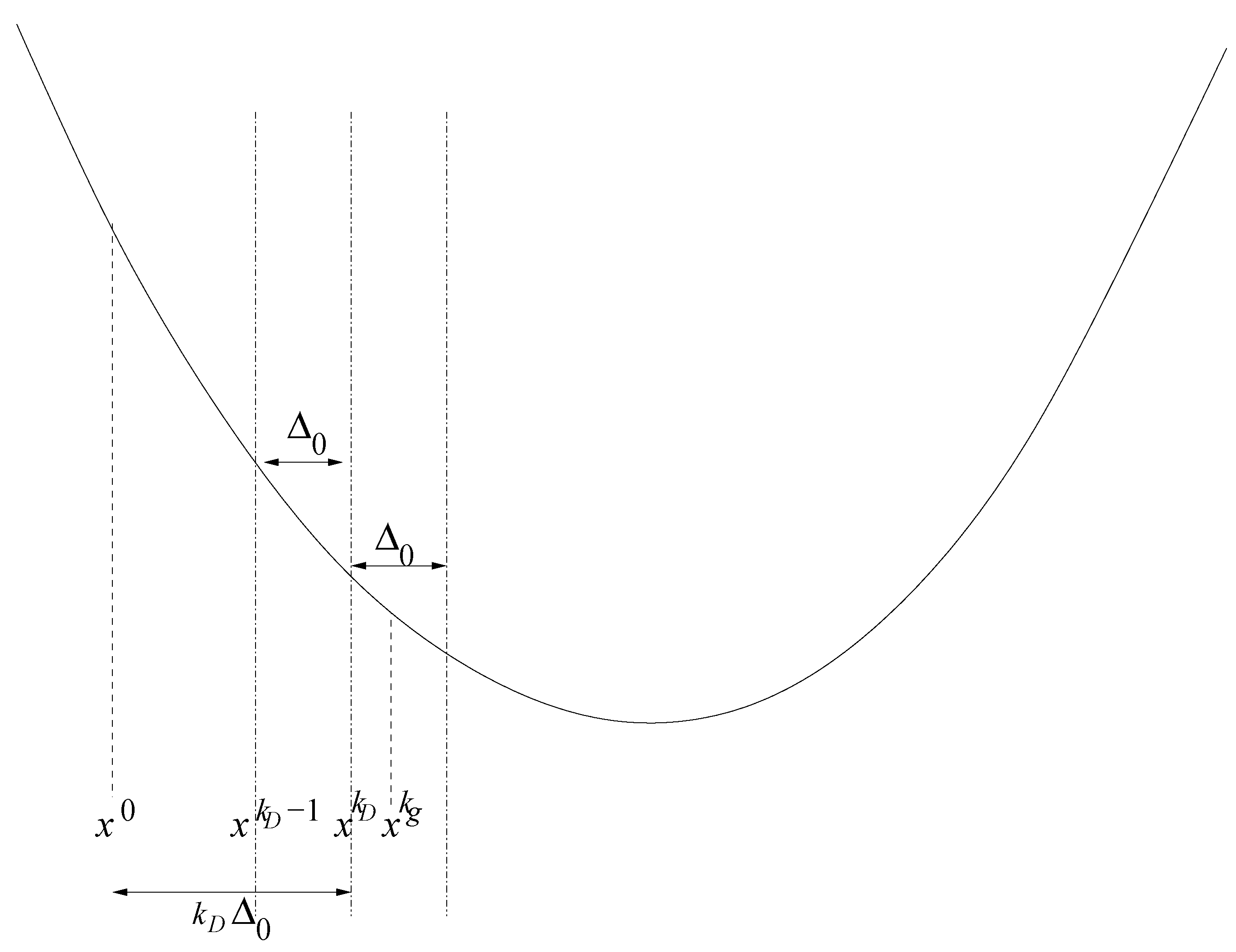
3.4. Speed of Convergency Compared to Gradient-Based Methods

The speed of convergency of SpaGrOW is discussed in the following, also with respect to statistical noise. As already mentioned, the trust region size, Δ, may not be too small, due to the noise. However, the convergency proof is based on the choice of a small Δ. This dilemma, which is also present in the case of gradient-based methods whenever two adjacent points are required for the computation of a partial derivative, leads to the need for an optimal parameterization of SpaGrOW. To achieve a high speed of convergency, primarily at the beginning of the optimization, the choice of a large Δ is required without hurting one of the assumptions for the convergency proof, cf. [40]. In the following, some heuristic considerations are made in this regard. Thereby, the index, g , refers to gradient-based descent methods, the index, H to descent methods using a Hessian and the index, S to SpaGrOW. Furthermore, let M ¯ be the average number of function evaluations per iteration and l ¯ , the average number of Armijo or Trust Region steps. Then, it holds:
M ¯ g = N + l ¯ g
M ¯ H = N + N ( N + 1 ) 2 + l ¯ H
M ¯ S = 2 N · l ¯ S
The drawback of SpaGrOW lies in the multiplicative dependency of M ¯ S on l ¯ S . This is due to the fact that a new sparse grid is used at each iteration step. However, at the beginning of the optimization, l ¯ g = l ¯ H = l ¯ S = 1 is assumed. Then, it holds M ¯ g < M ¯ S < M ¯ H . Hence, SpaGrOW requires less iterations on average than a method based on Hessians. However, in total, it has to manage with less iterations than a gradient-based method requiring less function evaluations per iteration: Let k be the general number of iterations; then it must hold: k S < k g . If:
k S < N + 1 2 N k g
SpaGrOW needs less iterations and function evaluations than a gradient-based method. Now, the question arises, how this can be steered. By choosing an initial Δ 0 (and also γ 1 ) that is large enough, a faster convergency can be achieved.
In the following, the initial phase of an optimization process is considered, and a short comparison between SpaGrOW and a gradient-based descent method is pointed out, i.e., it is discussed under what conditions the speed of convergency is significantly higher in the case of SpaGrOW. Please note that at the beginning of the optimization means here that the number of trust region or Armijo steps is equal to one at each iterations and that k g is chosen, so that the number of Armijo steps for x k g is still equal to one and for x k g + 1 , greater than one. Furthermore, choose k S , so that | | x k S - x 0 | | | | x k g - x 0 | | , the size of the trust region is equal to Δ 0 and x k g Ω k . Hence, x k g Ω k - 1 . This means that both x k S and x k g are reached by SpaGrOW with k S steps of length Δ 0 , which is depicted in Figure 11. The distance between x 0 and x k S is equal to k S Δ 0 . It holds:
k S Δ 0 | | x k g - x 0 | |
If:
Δ 0 > | | x k g - x 0 | | N + 1 2 N k g > 1 , if k g 2
i.e., if:
Δ 0 > ζ | | x k g - x 0 | |
for a maximal ζ ( 0 , 1 ) ; then, Inequality (62) follows. In practice, a realistic case is k g = 4 . If:
ζ : = 4 N ( N + 1 ) k g = N N + 1 < 1
is chosen, SpaGrOW requires less than 50% of the iterations and function evaluations required by the gradient-based descent method. Hence, a reduction of computation time by a factor of two is plausible at the beginning of the optimization process.
Figure 11. Speed of convergency of SpaGrOW at the beginning of the optimization. For an appropriate choice of the size of the initial trust region, Δ 0 , the number of iterations in the case of SpaGrOW ( k S ) is significantly smaller than in the case of a gradient-based method ( k g ). It is realistic that the number of iterations and function evaluations can be reduced by a factor of two.
Entropy 15 03640 g011

4. Practical Evaluation and Results

The methodology of SpaGrOW was implemented in python (version 2.4.3) and is modularly constructed. The software consists of a main control script and secondary control scripts for specific parts of the algorithm, e.g., for the sparse grid interpolations and the control of the smoothing procedures, which were implemented in S+ (version 2.1.10), scripting language related to the R Project for Statistical Computing [42].
The implementation of SpaGrOW contains the full algorithm described in the previous section and acts as an interface between optimization and simulation, providing all necessary control routines for both tasks. On the optimization side, the method starts with an initial guess and evaluates the loss function based on the results of a simulation. If one of the stopping criteria of SpaGrOW is fulfilled, the optimization workflow terminates. Otherwise, the parameters are updated by SpaGrOW.
On the simulation side, a control script calls the simulation tool performing all preparation routines and computing the trajectory, as well as the desired physical target properties. The latter are passed on to the optimization workflow of SpaGrOW. In the case of a simultaneous optimization of properties at different temperatures, the respective simulations are executed in parallel. In this case, a script distributing K jobs at K temperatures is called. A script controlling the parallel environment and the simulation control script are called K times. If m = n / K physical properties are fitted, the result of each job consists of m properties files. Figure 12 shows both the optimization and the simulation side and how they interact with each other in the case of parallel jobs at different temperatures.
Figure 12. Technical realization of optimization procedure for physical target properties at different temperatures. If the simulated properties do no coincide well with their experimental reference data, the optimization control script—depicted on the left—passes the current force field parameters on to a distribution control script, which submits parallel jobs at different temperatures. Then, a parallel environment control script is executed, and a simulation control script is called, which performs the following three tasks: preparation routines, the simulation itself and the computation of the simulated target properties. The properties are written into separate files, which are read by the optimization control script. Finally, the loss function is evaluated and the workflow continues.
Entropy 15 03640 g012
The simulations were performed on a parallel computer cluster with 215 available nodes, where each node is provided with two Intel-Nehalem-EP-Quadcore processors (Xeon X5550) with 24 GB of main storage, which are connected by a fast QDR infiniband interconnect with a 40-Gb/s Double Date Rate (DDR).
In this section, SpaGrOW is evaluated in practice and applied to molecular simulations as described above. The questions to be answered are the following:
  • Which smoothing and regularization procedure are most suitable?
  • Is SpaGrOW capable of saving simulations in comparison to gradient-based methods?
  • How close does SpaGrOW get to the minimum?

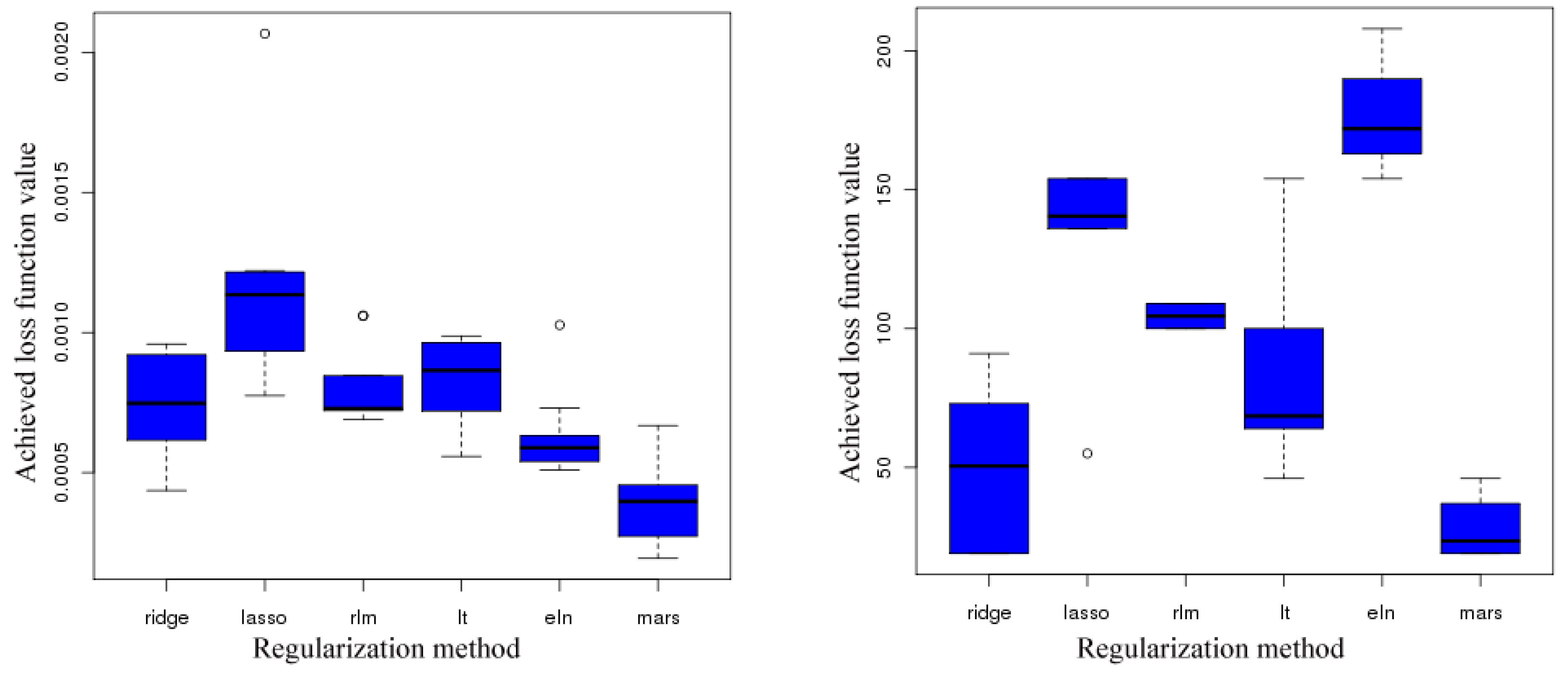
4.1. Selection of Smoothing and Regularization Methods

As molecular simulations are extremely time-consuming, an analytical model replacing them was used for the selection. In previous work [22], a similar assessment has already been performed for gradient-based methods. Vapor-Liquid Equilibrium (VLE) data, like the saturated liquid density, ρ l , the enthalpy of vaporization, Δ v H , and the vapor pressure, p σ , can be evaluated directly as functions of certain force field parameters. These functions were determined by [43] by nonlinear regression using a high amount of simulation data for two-centered Lennard-Jones (LJ) fluids with a quadrupolar moment. Here, nitrogen was considered as an example for this kind of fluid. The model parameters to be optimized were the elongation, L, of the two LJ sites, the quadrupolar moment, Q 2 , and the two LJ parameters, σ and ε. In order to mimic molecular simulations, uniformly distributed artificial uncertainties ( 0 . 5 % for the density and 3 % for the pressure) were added for the simultaneous optimization of ρ l and p σ at six different temperatures, T / K { 65 , 75 , 85 , 95 , 105 , 115 } . As in [22], the weights of the properties in the loss function were all equal to one, because all properties were considered as homologous. As the simulation data were noisy, ten statistically independent random replicates were performed for each optimization run, whose results were averaged.
Due to theoretical considerations, the tendency consists in selecting positive definite RBFs, in particular, Gaussian RBFs. In the following, it is shown that this is also a good choice in practice.
In order to evaluate, whether a smoothing or regularization procedure is appropriate for SpaGrOW, the behavior of the algorithm combined with each preprocessing procedure is analyzed. Thereby, both efficiency and robustness with respect to noise are considered. Table 2 shows the candidates and their abbreviations.
Table 2. Candidates for smoothing and regularization procedures within SpaGrOW together with their abbreviations.
Smoothing proceduresRegularization procedures
Radial Basis FunctionsLeast squares
Naive Elastic Nets (NENs)
α = 0 : Least Absolute Shrinkage and Selection Operator (LASSO)
α = 1 : Ridge Regression
Linear property approximation (Lipra)Multivariate Adaptive Regression Splines (MARS)
Figure 13. Box plots of the loss function values achieved by SpaGrOW in combination with a smoothing procedure based on Radial Basis Functions (RBFs). The RBFs were the linear, cubic, multiquadric (Multi), inverse multiquadric (Invers), Gaussian, thin plate spline RBF (TPS) and a Wendland function. Suitable RBFs were only the linear, cubic, Gaussian and thin plate spline RBF.
Entropy 15 03640 g013
Selection of the Best Smoothing Procedure It was already motivated that a smoothing procedure is indispensable, whenever noisy loss function values are present. A detailed analysis has shown that certain RBFs deliver better results by far than others. Suitable RBFs are the linear, cubic, Gaussian and thin plate spline RBF, cf. Section 2.2.2. The multiquadric functions were not reliable. Moreover, Wendland functions were considered, as well. Figure 13 shows box plots for the loss function values achieved by SpaGrOW combined with the different RBFs, which is a criterion for the quality of convergency. The results over ten statistically independent replicates are indicated. The lower the loss function achieved was, the closer got the algorithm to the minimum. The smallest loss function values were achieved robustly by the four RBFs mentioned above. A Gaussian RBF is selected here for the following reasons:
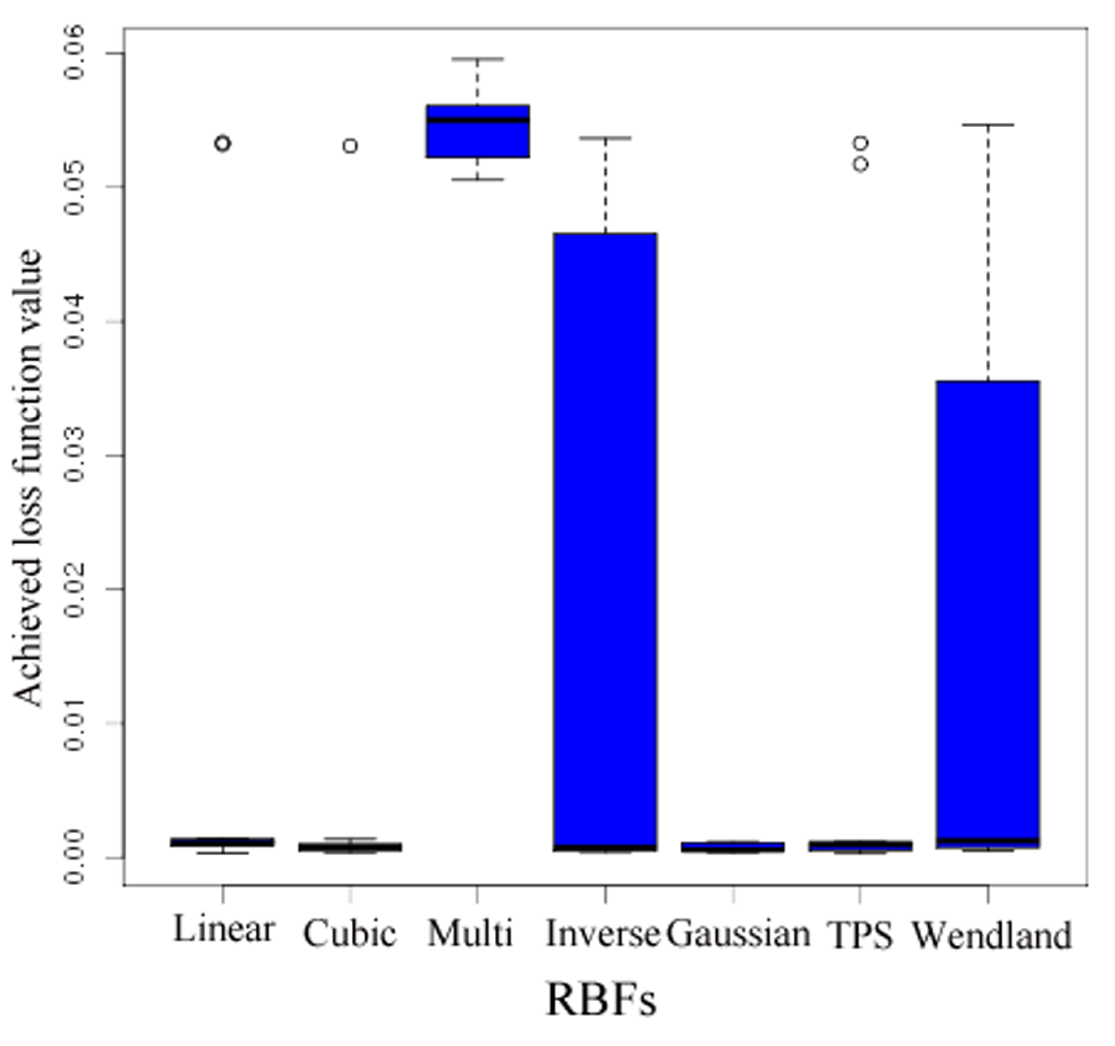
  • No outliers were detected.
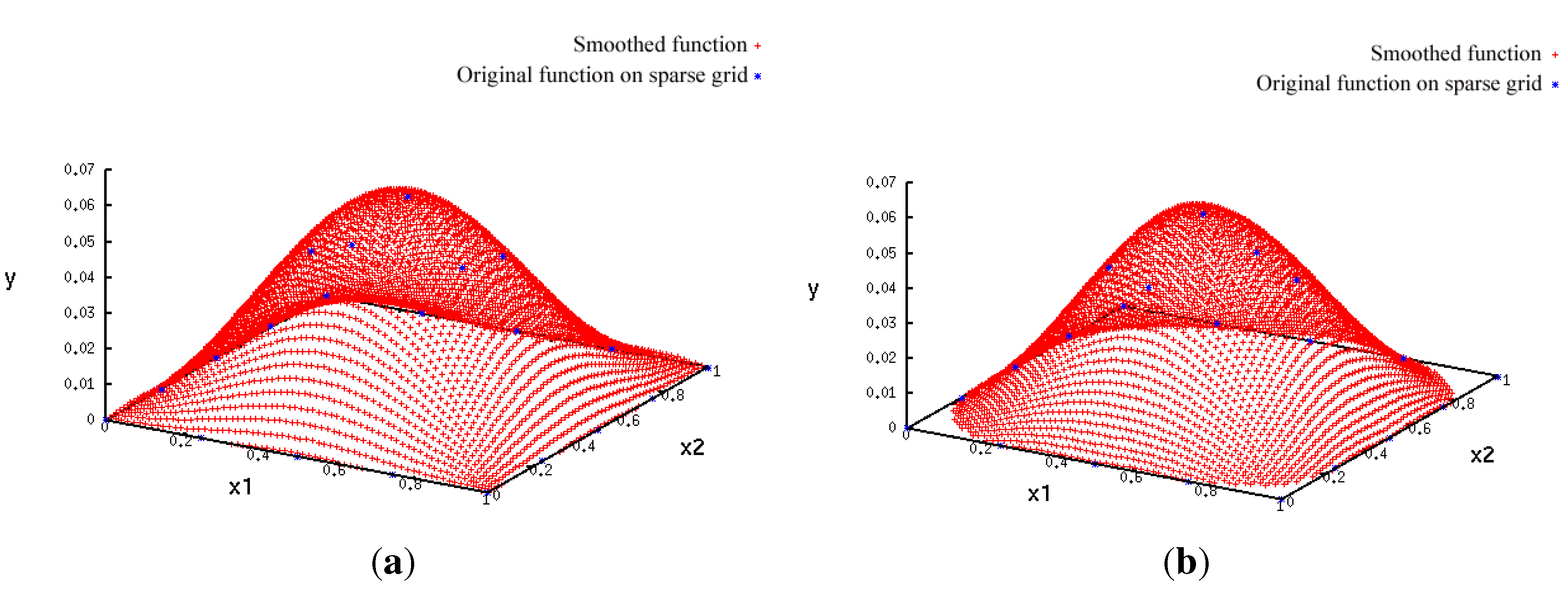
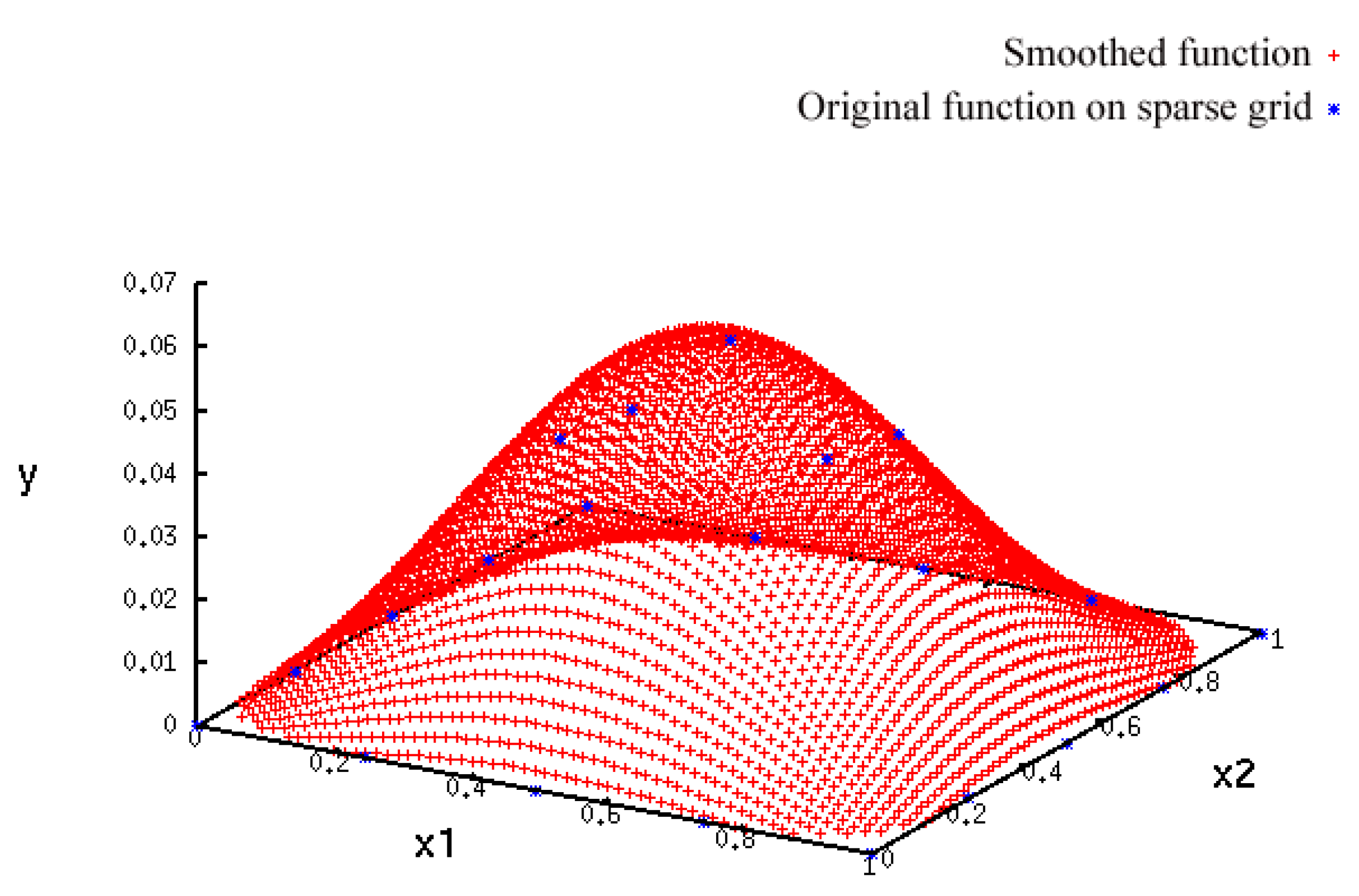
  • A more accurate analysis of the approximation error has shown that the smoothing procedures based on cubic and thin plate spline RBFs reproduced the function, F ¯ , cf. Section 3.2.1, worse than the one based on Gaussian RBFs. Figure 14 depicts the results for the Gaussian RBFs (Figure 14a) and the thin plate spline RBFs (Figure 14b) for the two-dimensional case: The approximating function and the original function values of F ¯ , cf. Equation (35), on a sparse grid of the level 2 are plotted versus ξ ( Q 2 ) and ξ ( L ) , cf. Equation (39). The LJ parameters, σ and ε, were fixed. As can be seen, a smoothing procedure based on thin plate spline RBFs reproduced F ¯ at the boundary of the unit square in a very bad fashion, whereas Gaussian RBFs delivered a good approximation on the complete unit square.
  • The Gaussian RBF is the only of the four RBFs mentioned above that is positive definite, i.e., the selection of Gaussian RBFs is also founded theoretically according to the considerations in Section 2.2.4.
Please note that linear RBFs delivered good approximations at the beginning of the optimization, as well, which was not surprising, because the steepest descent method was also very successful [22]. For higher dimensions, the Lipra method, i.e., a quadratic approximation of the loss function, could be convincing.
Figure 14. Approximations on the unit square, [ 0 , 1 ] 2 , based on Gaussian RBFs (a) and thin plate spline RBFs (b). The blue points mark the original (noisy) function values of F ¯ on the sparse grid. It holds x 1 = ξ ( Q 2 ) , x 2 = ξ ( L ) and y = F ¯ ( x 1 , x 2 ) . The smoothing procedure based on thin plate spline RBFs reproduces F ¯ at the boundary of the unit square in a very bad fashion.
Entropy 15 03640 g014
Selection of the Best Regularization Method As already mentioned, the selection of the best regularization method can only be achieved by practical evaluations. Candidates are least squares, NENs (LASSO for α = 0 and Ridge Regression for α = 1 ), as well as MARS.
The regularization methods were evaluated in combination with the selected smoothing procedure based on Gaussian RBFs. The application of least squares is the same as not using any regularization method. All other regularization methods could improve the results achieved with least squares only. The LASSO algorithm performs a variable selection, i.e., it tends to detect outliers by mistake. Hence, the model obtained by LASSO was often under-fitted. In contrast, the Ridge Regression estimator was more suitable for the present task, as it is a compromise between least squares, which often lead to overfitting, and the LASSO, which often leads to under-fitting. Figure 15 shows an approximation based on Gaussian RBFs in combination with LASSO. As can be seen, the function to be approximated was reproduced in a bad fashion at the boundary.
Figure 15. Approximations of F ¯ on the unit square, [ 0 , 1 ] 2 , based on Gaussian RBFs, combined with a LASSO regularization. The blue points mark the original (noisy) function values of F ¯ on the sparse grid. It holds x 1 = ξ ( Q 2 ) , x 2 = ξ ( L ) and y = F ¯ ( x 1 , x 2 ) . At the boundary of the unit square, the function is reproduced in a bad fashion.
Entropy 15 03640 g015
An NEN with α = 0 . 7 delivered an even better quality of convergence; however, the computational effort to optimize α was too high compared to the benefit achieved. The application of an NEN with α { 0 , 1 } is not worthwhile for the present task.
Figure 16. Box plots of the loss function values (a) and of the number of function evaluations (b) resulting from the application of SpaGrOW combined with a smoothing procedure based on Gaussian RBFs and different regularization methods: Ridge Regression, LASSO, a weighted linear regression (rlm), an RBF approximation with an additional linear term (lt), an NEN (eln) with α = 0 . 7 and MARS. It becomes clear that MARS is the algorithm to select for regularization. Ridge Regression is reliable, as well.
Entropy 15 03640 g016
The best regularization method is the MARS algorithm, not only with respect to robustness and quality of convergency, but also with respect to the number of function evaluations: Figure 16 shows box plots of all regularization methods applied. Figure 16a shows the loss function values achieved and Figure 16b the number of function evaluations. Besides the methods considered here, two other ones were tried: a weighted linear regression based on M-estimators and an RBF approximation with an additional linear term. As can be seen, the MARS algorithm delivers the best results. Hence, it is selected as regularization method for SpaGrOW. However, Ridge Regression is reliable, as well, and suggested as the alternative. The NEN with α = 0 . 7 achieved very low loss function values in a very robust way, but it always required more than a hundred function evaluations.
For Lipra, the least square estimator was the best regularization method. All other methods biased the quadratic approximation in a highly inappropriate way.
To summarize, Gaussian RBFs in combination with MARS and, in particular, for N 5 , the Lipra method together with the least square estimator have turned out to be most suitable for the present task and are implemented in SpaGrOW for this reason.

4.2. Application of SpaGROW to Molecular Simulations

Finally, SpaGrOW is applied to molecular simulations. Thereby, it is compared to gradient-based methods with respect to computational effort. Additionally, for an eight-dimensional problem, the Lipra method is evaluated, and it is analyzed how close SpaGrOW can get to the minimum.

4.2.1. Comparison to Gradient-Based Methods with Respect to Computation Time: Benzene and Ethylene Oxide

In the following, SpaGrOW is compared to GROW with respect to computational effort on the basis of two applications: benzene and ethylene oxide.
Benzene Benzene (C 6 H 6 ) is a quite simple molecule, because of its symmetric structure and the fact that it does not possess a permanent dipolar moment. Furthermore, benzene has two chemically independent atom types only. Hence, the force field parameterization for benzene was deemed to be a relatively easy task. However, it is still challenging, because of the π interactions.
Figure 17 shows the comparison between SpaGrOW and GROW with respect to the computational effort required within the respective optimization procedures. The target observables were the enthalpy of vaporization (Figure 17a) and the saturated liquid density (Figure 17b), considered at three different temperatures. The values indicated on the y-axis are the Mean Absolute Percentage Errors (MAPE), i.e., the absolute deviations from the respective experimental reference data in %, averaged over the range of temperatures. The experimental saturated liquid density was taken from [44] and the enthalpy of vaporization from the NISTdatabase [45]. The simulations performed were molecular dynamics simulations in the N p T ensemble executed with the software tool, GROMACS [46]. The non-bonded potential energy was computed by Moscito [47] using the trajectories collocated by GROMACS. Please note that the experimental target observables were VLE define data and that the simulated properties were only approximations, due to the lack of an explicit gas phase, which was assumed to be ideal. On the computer cluster mentioned above, three to four hours were required for the simulation of 1,000 benzene molecules for 2 ns using a time step of 2 fs. For SpaGrOW, the following variables were chosen: η 1 = 0 . 2 , η 2 = 0 . 7 , γ 1 = 0 . 5 , γ 2 = 1 . 1 , and Δ 0 = 0 . 3 × Δ max . The force field parameters were σ ( H ) , σ ( C ) , ε ( H ) and ε ( C ) . The initial parameters were taken from previous work [23]. Thereby, the saturated liquid density and the self-diffusion coefficient were optimized at the vapor-liquid coexistence curve. The feasible domain was defined as follows: σ was changed by no more than 30% and ε by no more than 80%. As it was a four-dimensional optimization problem, Gaussian RBFs were chosen for the smoothing and the MARS algorithm for the regularization procedure.
Figure 17. Mean Absolute Percentage Errors (MAPE) values with respect to Δ v H (a) and ρ l (b) for benzene during the SpaGrOW optimization in comparison to GROW. The smoothing procedure was based on Gaussian RBFs in combination with MARS. The force field parameters to be optimized were σ ( H ) , σ ( C ) , ε ( H ) and ε ( C ) . A faster convergency of SpaGrOW could be confirmed.
Entropy 15 03640 g017
GROW needed seven iterations in total: five steepest descent and two conjugate gradient iterations. In contrast, SpaGrOW required six iterations only. Please note that an optimal force field with respect to Δ v H and ρ l was already achieved after four iterations, i.e., both target observables were equal to their experimental reference data up to statistical uncertainties for all temperatures. Typical statistical uncertainties for Δ v H and ρ l are 1% and 0.5%, respectively, cf. e.g., [19]. For GROW, this was the case after seven iterations. The number of function evaluations, i.e., simulations, for SpaGrOW and GROW was 37 and 62, respectively. However, in the latter case, seven simulations have to be subtracted for the comparison, because the partial atomic charged were optimized, as well. Hence, in the case of GROW, it was a five-dimensional optimization problem, and for the gradient calculation, one simulation more was required at each iteration. However, SpaGrOW was significantly faster than GROW.
Figure 18 depicts the development of the LJ Parameters for GROW and SpaGrOW (Figure 18a refers to σ and Figure 18b to ε). σ ( C ) remained constant, and all other force field parameters were increased. At the fourth iteration of SpaGrOW, the parameters were very similar to the ones of GROW at the seventh iteration. However, the following interesting observation could be made. The parameter, σ ( C ) , remained constant, even during the whole optimization procedure. In the case of GROW, it was first decreased in order to obtain nearly the same value as before. As it is gradient-based, GROW tends to make detours. As it is grid-based, SpaGrOW is capable of keeping one or more parameters constant during the whole optimization procedure, because it can converge along a certain grid line or hyperplane. This is another reason for the faster convergency of SpaGrOW. Only in the case of ε, some small detours were observed. The algorithm ran through the triangle indicated in Figure 18b. SpaGrOW delivered a set of force field parameters, which differed a little from the ones obtained by GROW. Hence, it achieved a different domain close to the minimum.
Figure 18. Development of the Lennard-Jones (LJ) parameters in the case of benzene ( Δ v H , ρ l ) for GROW and SpaGrOW—σ(H) and σ(C) (a)—as well as ε(H) and ε(C) (b). The unfilled circles indicate the optimal parameters. SpaGrOW led in a more direct way to the minimum than GROW. Only in the case of ε, some detours could be observed, due to the triangle.
Entropy 15 03640 g018
Ethylene oxide Ethylene oxide (C 2 H 4 O) is a highly toxic substance, but very relevant for industrial applications, because it is an educt for many industrially fabricated materials. It is very suitable for the evaluations of the optimization algorithms, because it has been characterized both experimentally [48,49] and by molecular simulations [14,50,51].
Figure 19 shows the MAPE values for ethylene oxide during the optimization procedures. The target observables were the saturated liquid density (Figure 19a), the enthalpy of vaporization (Figure 19b) and the vapor pressure (Figure 19c), considered at seven different temperatures. For pressures, the statistical uncertainty within molecular simulations is higher than for Δ v H and ρ l . Here, 5% were assumed. Experimental data was taken from [48]. The simulations performed were Grand-Equilibrium Monte-Carlo (GEMC) simulations based on a rigid united-atom model with a dipolar moment developed by [14]. They were executed with the software tool ms2 [52]. As GEMC simulations simulate the liquid and gas phase successively, the VLE data could be calculated correctly. The liquid simulation was performed in the N p T ensemble and the gas simulation in the μVT ensemble, where the chemical potential, μ, was kept constant. On the computer cluster mentioned above, eight to ten hours were required for the simulation of 500 liquid and 500 gaseous ethylene oxide molecules. Thereby, the total number of 345,000 Monte-Carlo steps was distributed on eight processors. The force field parameters to be optimized were ε ( CH 2 ) , ε ( O ) , σ ( CH 2 ) and σ ( O ) . The initial parameters were the result of parameters obtained by a global pre-optimization based on random search [51]. Both parameters were changed by no more than 20%. The SpaGrOW variables were the same as for benzene. As the optimization problem was four-dimensional, Gaussian RBFs in combination with MARS were used again.
Figure 19. MAPE values with respect to ρ l (a), Δ v H (b) and p σ (c) in the case of ethylene oxide during the Vapor-Liquid Equilibrium (VLE) optimization for SpaGrOW and GROW. The smoothing procedure was based on Gaussian RBFs combined with the MARS algorithm. The force field parameters were ε ( CH 2 ) , ε ( O ) , σ ( CH 2 ) and σ ( O ) . The faster convergency of SpaGrOW compared to GROW could be confirmed again.
Entropy 15 03640 g019
In total, GROW required 14 iterations for the optimization using the steepest descent method only. SpaGrOW only needed five to achieve a comparable loss function value in the same order of magnitude: for GROW, F ( x ( 14 ) ) = 2 . 4 × 10 - 4 and, for SpaGrOW, F ( x ( 5 ) ) = 3 . 9 × 10 - 4 . Please note that the force field was not optimal and that other methods had to be applied in order to optimize it. For details, cf. [40]. SpaGrOW and GROW required 54 and 77 molecular simulations, respectively. Hence, SpaGrOW was significantly faster again.
Figure 20 shows the development of the LJ parameters during the optimization process in comparison to GROW (Figure 20a refers to ε and Figure 20b to σ). All parameters were decreased, and SpaGrOW delivered approximately the same parameters as GROW. Undesired detours were avoided again, except for σ. However, the detours made by GROW could be linearized.
Figure 20. Development of the LJ parameters in the case of ethylene oxide (VLE) for GROW and SpaGrOW: ε(CH 2 ) and ε(O) (a), as well as σ(CH 2 ) and σ(O) (b). The unfilled circles show the final parameters. SpaGrOW led to a more direct way to the minimum again.
Entropy 15 03640 g020
To summarize, SpaGrOW exhibits a significantly higher speed of convergency than GROW.

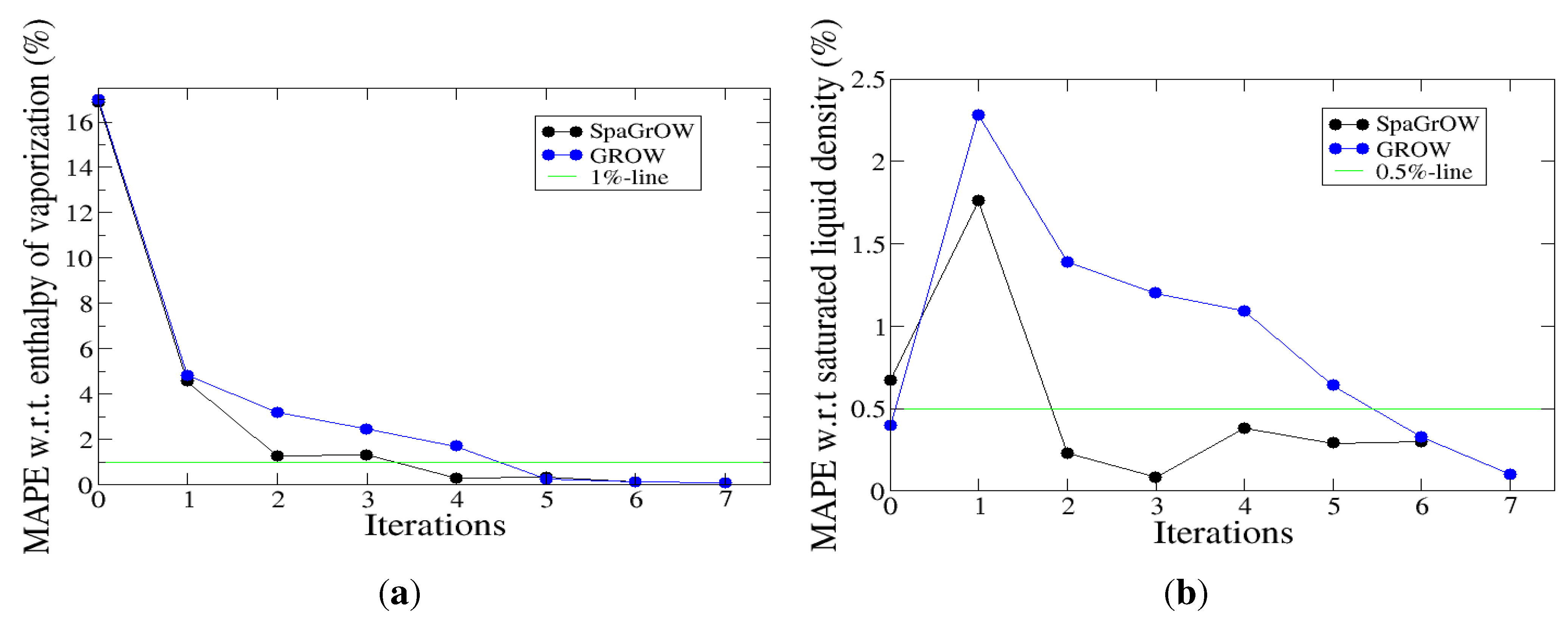
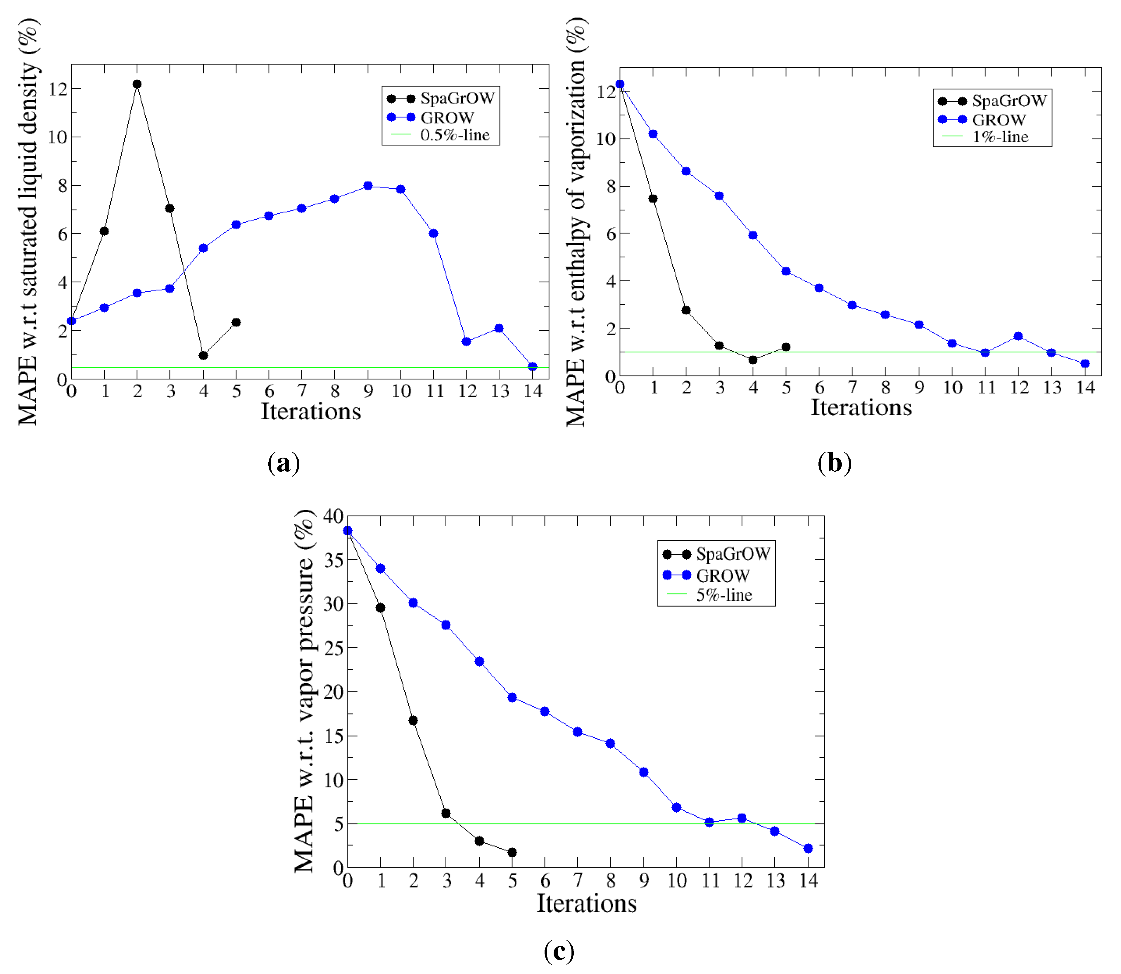
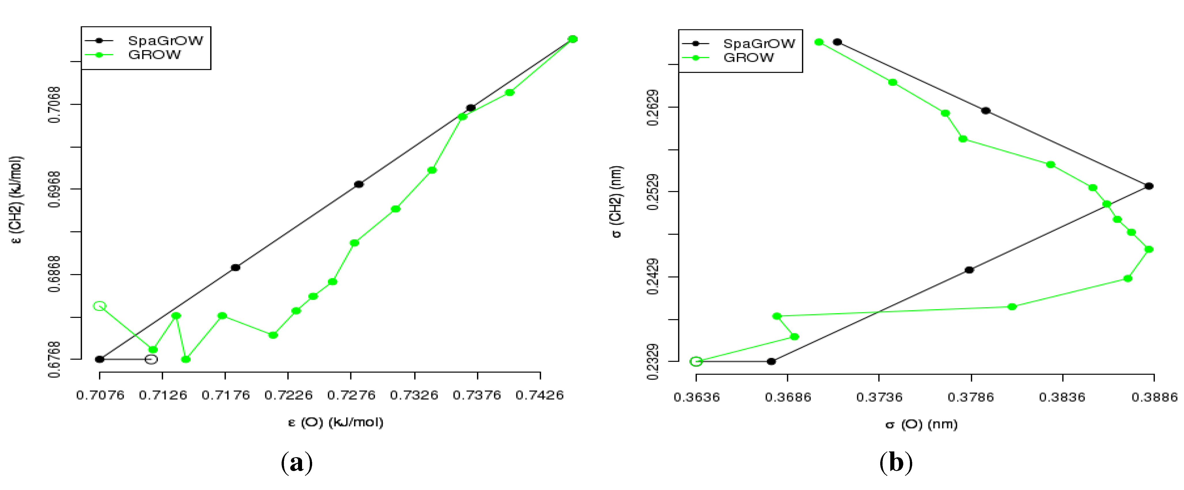
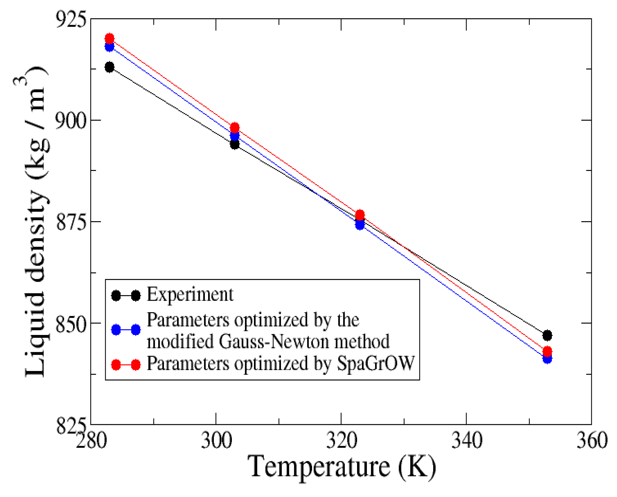
4.2.2. Comparison to Gradient-Based Methods Close to the Minimum: Dipropylene Glycol Dimethyl Ether

In the framework of the Industrial Fluid Property Simulation Challenge (IFPSC) 2010 [53], a liquid-liquid equilibrium (LLE) between two liquid phases should be calculated with molecular models. One of the two component was water and the other, dipropylene glycol dimethyl ether (C 8 H 18 O 3 ), an inert, water-resistant, nontoxic and industrially highly relevant solvent.
The target observable was the liquid density, ρ, only, considered at four different temperatures and taken from [54]. The simulations performed were molecular dynamics simulations in the N p T ensemble executed with the software tool, GROMACS [46]. On the computer cluster mentioned above, three to four hours were required for the simulation of 512 ether molecules for 0.5 ns using a time step of 2 fs.
The LJ sites were located at the CH 3 , the CH 2 , the CH group and the oxygen. Hence, it was an eight-dimensional optimization problem. The initial force field parameters from [55]. As GROW could not achieve an optimal force field reproducing the liquid density of the ether [55], another gradient-based method was applied, based on a Taylor series up to the first member for the target observables, delivering a quadratic model for the loss function. It is a modified Gauss-Newton method combined with the Trust Region approach, i.e., the quadratic model is minimized within a compact domain, as well. The algorithm has also been developed by the authors, cf. [40] for more details. After three iterations, the modified Gauss-Newton method could achieve optimal liquid densities.
Figure 21 indicates that SpaGrOW (with Δ 0 = 0 . 3 × Δ max ) required two iterations only to do so. As the optimization problem was eight-dimensional, the Lipra method was applied as a smoothing procedure. However, SpaGrOW needed 38 simulations, three-times more than the modified Gauss–Newton method, which only had to execute twelve simulations. With an optimal Δ 0 , the number of simulations could have been reduced to 19 in the case of SpaGrOW. The modified Gauss-Newton method is more reliable than SpaGrOW close to the minimum, but it could be shown that SpaGrOW is capable of getting closer to the minimum than the standard gradient-based algorithms used in GROW.
Figure 21. MAPE values with respect to ρ in the case of dipropylene glycol dimethyl ether during the optimization process of SpaGrOW in comparison to the modified Gauss-Newton method. The smoothing procedure was realized by the Lipra method. The optimization problem was eight-dimensional. SpaGrOW needed two iterations only, but significantly more simulations than the modified Gauss-Newton method in order to achieve optimal liquid densities.
Entropy 15 03640 g021
However, the Gauss-Newton method is only applicable close to the minimum, i.e., when the loss function is nearly quadratic. In contrast, SpaGrOW is more generally applicable, and another drawback of the Gauss-Newton method is that it requires a gradient, which is not guaranteed to be computable, due to the reasons mentioned in Section 1. Please note that the density is not as noisy as other target properties, like the pressure or diffusion coefficient. Of course, the existence of an optimal Δ for SpaGrOW is not guaranteed either in practice.
Figure 22 shows the optimal liquid densities as a function of temperature for the modified Gauss-Newton method and SpaGrOW. Both methods could achieve an optimal force field with respect to ρ in contrast to GROW. However, SpaGrOW could reproduce the trend of the curve better than the modified Gauss-Newton method.
To summarize, SpaGrOW is capable of getting closer to the minimum than GROW, when the smoothing procedure and Δ 0 are chosen properly. However, the modified Gauss-Newton method needs significantly less simulations.
Figure 22. Optimization of the density ρ in the case of dipropylene glycol dimethyl ether using the modified Gauss-Newton method and SpaGrOW. Optimal densities could be achieved by both methods, but SpaGrOW needed many more simulations. However, SpaGrOW could reproduce the trend of the curve better.
Entropy 15 03640 g022

5. Conclusions

In this paper, the new derivative-free optimization method was presented in detail and applied to the parameterization of force fields in the field of molecular simulations. It is a combination of appropriate smoothing and regularization procedures, interpolation on sparse grids and the Trust Region approach. SpaGrOW turned out to be a highly efficient algorithm outperforming standard gradient-based methods with respect to the speed of convergency. Furthermore, it is capable of getting closer to the minimum. However, if a gradient can be calculated correctly, the gradient-based methods exhibit a slightly higher robustness than SpaGrOW. The new method is validated in the following with respect to the three criteria speed of convergency, local refinements and robustness:
  • Speed of convergency: Whenever Δ 0 is chosen properly, SpaGrOW often requires only half of the number of simulations than gradient-based methods. The speed of convergency was also higher, i.e., the number of iterations was significantly lower.
    The choice, Δ 0 = 0 . 3 × Δ max , was suitable in most cases, i.e., the parameterization of SpaGrOW is not critical at the beginning of the optimization.
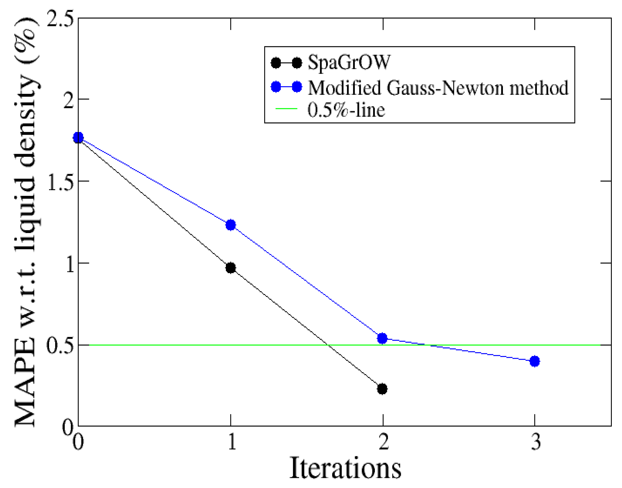
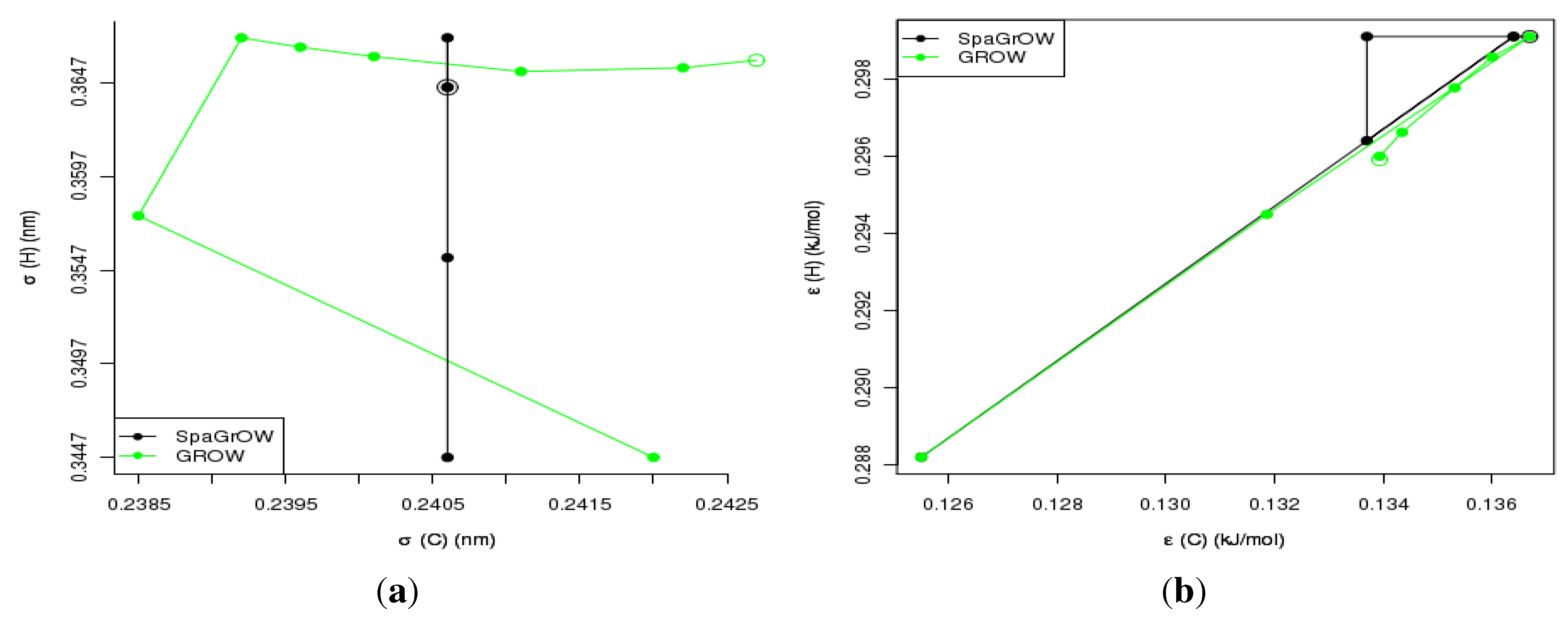
  • Local refinements: SpaGrOW is capable of getting closer to the minimum than GROW. However, the choice of Δ becomes critical, which reduces the robustness of SpaGrOW: If Δ is too high, the smoothing and interpolation algorithms cannot deliver a reliable model for the loss functions. If it is too small, only noise can be reproduced. A modified Gauss-Newton method turned out to be more efficient and close to the minimum, if the associated gradients can be computed correctly. An important advantage of SpaGrOW is the fact that the step length can be modified by the Trust Region steps, leading to different descent directions, which is not possible for gradient-based methods first determining the descent direction and, then, searching for a reliable step length.
  • Robustness: SpaGrOW exhibits a slightly lower robustness than the gradient-based methods. Due to an inappropriate choice of Δ, the minimum of the model can be transferred under certain conditions, and the course of the algorithm can be modified. The variable must be chosen, so that a decreasing trend of the loss function is present within the actual trust region. However, this is not trivial here, because the shape of the loss function is not known a priori.
It is extremely difficult to find a method that is efficient and robust at the same time. These two properties often face each other: Stochastic global optimization methods, like simulated annealing or evolutionary algorithms, are very robust with respect to statistical noise, but require a high amount of computation time to determine the global minimum exactly. Gradient-based ones are fast-convergent, but are less robust and reliant on the differentiability of the function to be minimized. SpaGrOW is situated in between: The higher speed of convergency has to be compensated by a lower robustness. However, the robustness was not reduced significantly, and the assumption that the loss function is smooth does not have to be made. Furthermore, SpaGrOW may still be successful when gradient-based methods exist.
To summarize, SpaGrOW is a generic, efficient and, also, quite robust algorithm, which can be used for many optimization problems. For force field parameterization tasks, it is highly recommended and preferred to gradient-based algorithms.

Acknowledgements

We are grateful to Janina Hemmersbach for the detailed analysis and selection of appropriate smoothing procedures, as well as to Anton Schüller for fruitful discussions and advice.

Conflicts of Interest

The authors declare no conflict of interest.

References

  1. Allen, M.P.; Tildesley, D.J. Computer Simulation of Liquids; Clarendon Press: Oxford, UK, 1987. [Google Scholar]
  2. Frenkel, D.; Smit, B. Understanding Molecular Simulation: From Algorithms to Applications; Academic Press: Waltham, MA, USA, 2006. [Google Scholar]
  3. Schrödinger, E. Quantisierung als eigenwertproblem. Ann. Phys. 1926, 79, 361–367. [Google Scholar] [CrossRef]
  4. Jensen, F. Introduction to Computational Chemistry; Wiley: Hoboken, NJ, USA, 1999. [Google Scholar]
  5. Guevara-Carrion, G.; Hasse, H.; Vrabec, J. Multiscale Molecular Methods in Applied Chemistry; Kirschner, B., Vrabec, J., Eds.; Series: Topics in Current Chemistry; Volume 307, Springer: Berlin/Heidelberg, Germany, 2012; pp. 201–249. [Google Scholar]
  6. Weiner, S.J.; Kollman, P.A.; Case, D.A.; Singh, U.C.; Ghio, C.; Alagona, G.; Profeta, S.; Weiner, P. A new force field for molecular mechanical simulation of nucleic acids and proteins. J. Am. Chem. Soc. 1984, 106, 765–784. [Google Scholar] [CrossRef]
  7. Berendsen, H.J.; van Gunsteren, W.F. GROMOS87 Manual; Library Manual; Biomos AG: Groningen, The Netherlands, 1987. [Google Scholar]
  8. Jorgensen, W.L.; Maxwell, D.S.; Tirado-Rives, J. Development and testing of the OPLS all-atom force field on conformational energetics and properties of organic liquids. J. Am. Chem. Soc. 1996, 118, 11225–11236. [Google Scholar] [CrossRef]
  9. Duan, Y.; Wu, C.; Chowdhury, S.; Lee, M.C.; Xiong, G.; Zhang, W.; Yang, R.; Cieplak, P.; Luo, R.; Lee, T.; et al. A point-charge force field for molecular mechanics simulations of proteins based on condensed-phase quantum mechancical calculations. J. Comput. Chem. 2003, 24, 1999–2012. [Google Scholar] [CrossRef] [PubMed]
  10. Reith, D.; Kirschner, K.N. A modern workflow for force-field development—bridging quantum mechanics and atomistic computational models. Comput. Phys. Commun. 2011, 182, 2184–2191. [Google Scholar] [CrossRef]
  11. Kräemer-Fuhrmann, O.; Neisius, J.; Gehlen, N.; Reith, D.; Kirschner, K.N. Wolf2Pack—Portal based atomistic force-field development. J. Chem. Inf. Mod. 2013, 53, 802–808. [Google Scholar] [CrossRef] [PubMed]
  12. Jorgensen, W.L.; Madura, J.D.; Swensen, C.J. Optimized intermolecular potential functions for liquid hydrocarbons. J. Am. Chem. Soc. 1984, 106, 6638–6646. [Google Scholar] [CrossRef]
  13. Martin, M.G.; Siepmann, J.I. Transferable potentials for phase equilibria. 1. United-atom description of n-alkanes. J. Phys. Chem. B 1998, 102, 2567–2577. [Google Scholar] [CrossRef]
  14. Eckl, B.; Vrabec, J.; Hasse, H. On the application of force fields for predicting a wide variety of properties: Ethylene oxide as an example. Fluid Phase Equilib. 2008, 274, 16–26. [Google Scholar] [CrossRef]
  15. Peguin, R.P.S.; Kamath, G.; Potoff, J.J.; da Rocha, S.R.P. All-atom force field for the prediction of vapor–liquid equilibria and interfacial properties of HFA134a. J. Phys. Chem. B 2009, 113, 178–187. [Google Scholar] [CrossRef] [PubMed]
  16. Faller, R.; Schmitz, H.; Biermann, O.; Müller-Plathe, F. Automatic parameterization of force fields liquids by simplex optimization. J. Comput. Chem. 1999, 20, 1009–1017. [Google Scholar] [CrossRef]
  17. Ungerer, P.; Beauvais, C.; Delhommelle, J.; Boutin, A.; Rousseau, B.; Fuchs, A.H. Optimization of the anisotropic united atoms intermolecular potential for n-alkanes. J. Comput. Phys. 1999, 112, 5499–5510. [Google Scholar] [CrossRef]
  18. Bourasseau, E.; Haboudou, M.; Boutin, A.; Fuchs, A.H.; Ungerer, P. New optimization method for intermolecular potentials: Optimization of a new anisotropic united atoms potential for Olefins: Prediction of equilibrium properties. J. Chem. Phys. 2003, 118, 3020–3034. [Google Scholar] [CrossRef]
  19. Stoll, J.; Vrabec, J.; Hasse, H. A set of molecular models for carbon monoxide and halogenated hydrocarbons. J. Chem. Phys. 2003, 119, 11396–11407. [Google Scholar] [CrossRef]
  20. Sun, H. Prediction of fluid densities using automatically derived VDW parameters. Fluid Phase Equilib. 2004, 217, 59–76. [Google Scholar] [CrossRef]
  21. Hülsmann, M.; Köddermann, T.; Vrabec, J.; Reith, D. GROW: A gradient-based optimization workflow for the automated development of molecular models. Comput. Phys. Commun. 2010, 181, 499–513. [Google Scholar] [CrossRef]
  22. Hülsmann, M.; Vrabec, J.; Maaß, A.; Reith, D. Assessment of numerical optimization algorithms for the development of molecular models. Comput. Phys. Commun. 2010, 181, 887–905. [Google Scholar] [CrossRef]
  23. Hülsmann, M.; Müller, T.J.; Köddermann, T.; Reith, D. Automated force field optimisation of small molecules using a gradient-based workflow package. Mol. Simul. 2011, 36, 1182–1196. [Google Scholar] [CrossRef]
  24. Griebel, M.; Schneider, M.; Zenger, C. A Combination Technique for the Solution of Sparse Grid Problems; Technical Report; Institut für Informatik, Technische Universität München: Munich, Germany, 1990. [Google Scholar]
  25. Moré, J.J. Mathematical Programming: The State of the Art; Bachem, A., Grötschel, M., Korte, B., Eds.; Springer: Berlin/Heidelberg, Germany, 1983; pp. 258–287. [Google Scholar]
  26. Nocedal, J.; Wright, S.J. Numerical Optimization; Springer: Berlin/Heidelberg, Germany, 1999. [Google Scholar]
  27. Mangasarian, O.L.; Rosen, J.B.; Thompson, M.E. Global minimization via piecewise-linear underestimation. J. Glob. Optim. 2004, 32, 1–9. [Google Scholar] [CrossRef]
  28. Smolyak, S.A. Quadrature and interpolation formulas for tensor products of certain classes of functions. Sov. Math. Doklady 1963, 4, 240–243. [Google Scholar]
  29. Zenger, C. Parallel Algorithms for Partial Differential Equations, Notes on Numerical Fluid Mechanics; Hackbusch, W., Ed.; Vieweg: Wiesbaden, Germany, 1991; Volume 31, pp. 241–251. [Google Scholar]
  30. Bungartz, H.-J. Iterative Methods in Linear Algebra. In Proceedings of the IMACS International Symposium, Brüssel, Belgium, April 1991; de Groen, P., Beauwens, R., Eds.; North-Holland Publishing Co.: Amsterdam, The Netherlands, 1992; pp. 293–310. [Google Scholar]
  31. Powell, M. Algorithms for Approximation; Mason, J.C., Cox, M.G., Eds.; Clarendon Press: Oxford, UK, 1987; pp. 143–167. [Google Scholar]
  32. Bishop, C.M. Pattern Recognition and Machine Learning; Series: Information Science and Statistics; Springer: Berlin/Heidelberg, Germany, 2007. [Google Scholar]
  33. MacQueen, J.B. Some Methods for Classification and Analysis of Multivariate Observations. In Proceedings of the 5th Berkeley Symposium on Mathematical Statistics and Probability, Berkeley, CA, USA, June/July 1965; University of California Press: Berkeley, CA, USA, 1967; pp. 281–297. [Google Scholar]
  34. Zou, H.; Hastie, T. Regularization and variable selection via the elastic net. J. Roy. Stat. Soc. Ser. B 2005, 67, 301–320. [Google Scholar] [CrossRef]
  35. Hoerl, A.E.; Kennard, R.W. Ridge regression: Biased estimation for nonorthogonal problems. Technometrics 1970, 12, 55–67. [Google Scholar] [CrossRef]
  36. Tibshirani, R. Regression shrinkage and selection via the lasso. J. Roy. Stat. Soc. Ser. B 1996, 58, 267–288. [Google Scholar]
  37. Friedman, J.H. Multivariate adaptive regression splines. Ann. Stat. 1991, 19, 1–67. [Google Scholar] [CrossRef]
  38. Wendland, H. Scattered Data Approximation; Cambridge University Press: Cambridge, UK, 2005. [Google Scholar]
  39. Wendland, H. Konstruktion und Untersuchung radialer Basisfunktionen mit kompaktem Träger. Ph.D. Thesis, Universität Göttingen, Göttingen, Germany, 1996. [Google Scholar]
  40. Hülsmann, M. Effiziente und neuartige Verfahren zur Optimierung von Kraftfeldparametern bei atomistischen Molekularen Simulationen kondensierter Materie. Ph.D. Thesis, Universität zu Köln, Cologne, Germany, 2012. [Google Scholar]
  41. Conn, A.R.; Scheinberg, K.; Toint, P.L. On the Convergence of Derivative-free Methods for Unconstrained Optimization; Iserles, A., Buhmann, M., Eds.; Cambridge University Press: Cambridge, UK, 1997. [Google Scholar]
  42. The R Project for Statistical Computing. Available online: http://www.r-project.org/ (accessed on 14 February 2013).
  43. Stoll, J.; Vrabec, J.; Hasse, H.; Fischer, J. Comprehensive study of the vapour-liquid equilibria of the pure two-centre Lennard-Jones plus pointquadrupole fluid. Fluid Phase Equilib. 2001, 179, 339–362. [Google Scholar] [CrossRef]
  44. Yoshida, K.; Matubayasi, N.; Nakahara, M. Self-diffusion coefficients for water and organic solvents at high temperatures along the coexistence curve. J. Chem. Phys. 2008, 129, 214501–214509. [Google Scholar] [CrossRef] [PubMed]
  45. NIST Chemistry Webbook. Available online: http://webbook.nist.gov/chemistry/ (accessed on 14 February 2013).
  46. GROMACS Molecular Simulation Tool. Available online: http://www.gromacs.org/ (accessed on 14 February 2013).
  47. Moscito Molecular Simulation Tool. Available online: http://ganter.chemie.uni-dortmund.de/MOSCITO/ (accessed on 14 February 2013).
  48. Buckles, C.; Chipman, P.; Cubillas, M.; Lakin, M.; Slezak, D.; Townsend, D.; Vogel, K.; Wagner, M. Ethylene Oxide User’s Guide; Online Manual, Publisher; American Chemistry Council, 1999; Available online: http://www.ethyleneoxide.com (accessed on 14 February 2013).
  49. Olson, J.D.; Wilson, L.C. Benchmarks for the fourth industrial fluid properties simulation Challenge. Fluid Phase Equilib. 2008, 274, 10–15. [Google Scholar] [CrossRef]
  50. Müller, T.J.; Roy, S.; Zhao, W.; Maaß, A.; Reith, D. Economic simplex optimization for broad range property prediction: Strengths and weaknesses of an automated approach for tailoring of parameters. Fluid Phase Equilib. 2008, 274, 27–35. [Google Scholar] [CrossRef]
  51. Maaß, A.; Nikitina, L.; Clees, T.; Kirschner, K.N.; Reith, D. Multiobjective optimisation on the basis of random models for ethylene oxide. Mol. Simul. 2010, 36, 1208–1218. [Google Scholar] [CrossRef]
  52. ms2 Molecular Simulation Tool. Available online: http://www.ms-2.de/ (accessed on 14 February 2013).
  53. The Industrial Fluid Property Simulation Challenge. 2010. Available online: http://www.ifpsc.com (accessed on 14 February 2013).
  54. Esteve, X.; Conesa, A.; Coronas, A. Liquid densities, kinematic viscosities, and heat capacities of some alkylene glycol dialkyl ethers. J. Chem. Eng. Data 2003, 48, 392–397. [Google Scholar] [CrossRef]
  55. Köddermann, T.; Kirschner, K.N.; Vrabec, J.; Hülsmann, M.; Reith, D. Liquid-liquid equilibria of dipropylene glycol dimethyl ether and water by molecular dynamics. Fluid Phase Equilib. 2011, 310, 25–31. [Google Scholar] [CrossRef]

