1. Introduction
The increased water pollution due to the inflow of diverse pollutants into groundwater, lakes, rivers and seas caused by industrialization has necessitated the establishment of water pollution monitoring networks and the operation of continuous monitoring for effective water quality management. Since the 1970s, rapid industrialization has led to serious water pollution problems in Korea. In response, the Korean government has established a network of water quality monitoring points in rivers, raw water, lakes, marshes and urban streams for water quality management. Similarly, continuous monitoring of the sewer system for efficient management of water quantity and quality in conduits as well as infiltration and inflow has become more important.
Sanders
et al. [
1], Ward
et al. [
2], Harmancioglu
et al. [
3] and Strobl and Robillard [
4] produced an overview of the current network design procedures and developed basic guidelines to be followed in both the design and the redesign of water quality monitoring networks. Their studies treat the network design problem in a comprehensive and systematic framework, starting with objectives of monitoring and elaborating on various technical design features, e.g., selection of sampling sites, sampling frequencies, variables to be monitored, and sampling duration. Khalil and Ouarda [
5] reviewed the statistical approaches utilized for the assessment and redesign of surface water quality monitoring (WQM) networks and Khalil
et al. [
6] explained the various deficiencies in the statistical approaches proposed in the literature for the assessment and redesign of surface WQM locations. Beveridge
et al. [
7] used geostatistical methods to quantify redundancy in an intentionally dense network of lake stations. Two statistical approaches (kriging and Local Moran’s I) were used to assess redundancy and these techniques identified stations that were statistically important or redundant. Ou
et al. [
8] developed a flexible and comprehensive framework for the selection of multiple sampling locations of multiple variables which was accomplished by coupling geostatistical approaches with principal component analysis (PCA) and fuzzy optimal model (FOM). Amirabdollahian and Datta [
9] reviewed different source identification and monitoring network design methods in groundwater contaminant sites. However, these studies dealt mainly with the assessment and design of water quality monitoring networks for the natural watershed such as lake, river and stream. There has been no study on the sewer system for the design of water quality monitoring networks.
To establish water quality monitoring networks within budget constraints, water quality monitoring points that can maximize the monitoring effect for a given cost must be selected. Meyer
et al. used a simulated annealing approach to solve the multi-objective integer programming of optimal monitoring network design [
10]. Hudak defined the configuration of monitoring wells for a solid water landfill in Tarrant County, TX, USA. The objective of investigation was to design a monitoring network which is able to minimize the undetected contaminant plumes in the study area [
11]. Dhar and Datta [
12] proposed a chance-constrained single and multi-objective nonlinear optimization models which are capable of designing optimal time variant groundwater quality monitoring network. Park
et al. [
13] used the genetic algorithm (GA) for the design of a water quality monitoring network. Wang
et al. [
14] studied an object-oriented design plan to improve the water quality monitoring network of the Han River. However, there has been no study on the establishment of an optimum water quality monitoring network for a sewer system. This research proposes a design method for the establishment of an optimal water quality monitoring network in a sewer system under budget constraints.
Entropy theory was applied to generate standards for the assessment of the optimal water quality monitoring network. The entropy theory considers the trans-information among both locations where water quality monitoring facilities are installed and locations without such facilities. Therefore, the theory can support the establishment of the water quality monitoring network by reducing the uncertainty on the basis of information produced by the network. Entropy is a measure of the degree of uncertainty of random hydrological processes. It is also a quantitative measure of the information content of a series of data since reduction of uncertainty, by making observations, equals the same amount of gain in information [
15]. Multivariate trans-information, which is one of the variates defined by the entropy theory, can be referred to as the information transmission and also called the mutual information. The multivariate entropy measures can then be used to assess the basic features in a network,
i.e., sampling sites, sampling frequencies, variables sampled and sampling duration [
3]. Therefore, many studies across diverse fields have sought to determine the combinations of assessment points that maximize the multivariate trans-information. Examples include the design of a precipitation monitoring network [
16,
17] and the assessment of a water quality monitoring network in river streams [
18,
19]. These studies however used the inefficient trial and error method in searching for the combinations that maximize the information transfer. With increasing number of combinations more sophisticated optimization methods are needed. The existing studies have mainly dealt with the assessment and design of a water quality monitoring network in natural basins such as lakes and rivers. Only tens of monitoring points are the object of analysis in the natural basins, but tens to hundreds of manhole points are the object of analysis in a network of urban sewer system. Therefore, the number of cases of combinations of monitoring points can be innumerable in sewer networks unlike in lakes or rivers, so the application of an optimization technique is necessary to find an optimal combination effectively.
With the aim of solving these issues, this research proposes a model for selecting optimized water quality monitoring points of sewer network system. The entropy variates are applied to the quantitative assessment in the selection of the optimal water quality monitoring points. An optimization method using a genetic algorithm (GA) is proposed to select optimized water quality monitoring points that can efficiently collect the maximum amount of data when the number of such water quality monitoring points is restricted because of budget constraints.
2. Entropy Measures
In classical thermodynamics, entropy is the quantity determined by the thermal condition in a physical system, which expresses the possibility of converting a given amount of heat into work [
20]. From the perspective of statistical thermodynamics, entropy refers to the statistical thermodynamic degree of disorder or uncertainty [
21]. In information theory, entropy is defined as the quantity of information possessed by a signal [
22]. This concept of entropy defined in information theory is used in this study.
In a definition adopted from information theory, entropy is the numerical expression of information on signals inside a system. In using this concept, the process of information exchange is as important as the amount of information. Information exchange occurs as signals are sent and statistically the extent of embedded uncertainty is reduced with increasing quantity of information in the signals. Therefore, the quantity of information can be measured indirectly based on the degree of the reduction of uncertainty, i.e., the larger entropy means a greater reduction of the uncertainty in a specific location.
In information theory, variates such as marginal entropy (Shannon entropy), conditional entropy, and trans-information are defined for the quantification of entropy. Firstly, marginal entropy
is defined as follows for the discrete random variate
[
22]:
where,
is the probability distribution of
where
and
are the lower and upper limits of
, respectively. The number of variate
that belongs to the scope of
is
. The total of probability values in the scope should be 1,
i.e.,
. If
is defined as the continuous random variate that follows the probability density function
, the marginal entropy is defined as follows [
23]:
The conditional entropy
of the two given continuous random variates
and
can be interpreted as the information loss that occurs during the trans-information process between
and
under a given condition. Equation (3) is the result of the application of the concept of conditional probability density function
[
23].
Amorocho and Espildora proposed that the marginal entropy can be expressed as the following when the continuous variate
is divided by the pre-determined interval
[
24]:
Moreover, Chapman proposed the conditional entropy when
and
are divided by the fixed interval
[
25]:
Here,
refers to the joint probability density function of
and
. The trans-information between the two continuous random variates
and
points to the reduction of uncertainty of
when
is given as Equation (6) [
24]:
The conditional entropy and trans-information presented above illustrate cases with two variates. These can be generalized for independent variables
with
as the number of variables [
26].
To obtain entropy variates from the water quality data time series used in this study, it is necessary to know probability density function f(
based on continuous random variable
X. The FARD2006 model, jointly developed by the National Institute for Disaster Prevention and Yonsei University was used for the goodness of fit test of the water quality determinand of Total Suspended Solids (TSS). To estimate the statistical parameters, the method of moment was used. The results of the
test and the Kolmogorov-Smirnov (K-S) test confirmed that the water quality data to be used was subject to the lognormal distribution. For lognormal distributions, Amorocho and Espildora proposed equations for estimating the marginal entropy, conditional entropy, and trans-information of multivariate
, which is divided by the regular interval
[
24]. Based on the equation, Chapman applied
, which is proportional to the scope of the variables, to produce Equations (7) and (8) for the marginal entropy and conditional entropy, respectively [
25].
where,
is the standard deviation of
and
the correlation coefficient of
and
. From Equations (6) through (8), the trans-information can be derived as follows [
25]:
3. Model for Selecting Optimal Water Quality Monitoring Points
In this study, the entropy theory was applied to the selection of the water quality monitoring points in a sewer system. Equation (6) expresses the trans-information between two variates. In the case of the sewer system, the number of candidate locations for the installation of water quality monitoring facilities is mostly more than two. Hence, Equation (6) should be expanded as an equation for more variates. In this study, the multivariate trans-information equation [Equation (10)], developed by Al-Zahrani and Husain [
17] for the selection of precipitation monitoring locations in the natural stream basin, was used for the selection of water quality monitoring points:
where,
is the total number of water quality monitoring locations that can be installed in the basin and
is the combination of the selected locations. The selected locations
form the combination that maximize
, the trans-information of the selected locations.
is the total of the marginal entropy of the selected water quality monitoring locations and
is the total of the trans-information between the selected locations and the locations that were not selected. Alternatively, the sum can be defined as the amount of information on unselected locations that can be obtained from the selected water quality monitoring points.
In this study, the objective function is defined to search the combination of positions that maximize the multi-location trans-information
as:
A constraint is that all entropy variates (marginal entropy, trans-information, etc.) have positive values.
If only one monitoring point should be selected, a point with the biggest trans-information value shall be selected. However, if two monitoring points are maintained, those points cannot be determined by simply comparing the trans-information obtainable from each point. This is because the trans-informations between the selected monitoring points and the remaining points differ depending on the choice of monitoring points. That is, when selecting any two points, it shall be determined so that the Itotal value may be maximized by considering the relationship between the selected points and the remaining points. Accordingly, when selecting n points for a total of m points, the entropy values for mCn combinations should be calculated to select the best combination with the maximum Itotal. Then, in sewer networks, a network contains tens to hundreds of manhole points in general. Therefore, the number of cases of combinations to calculate the value of Itotal increases geometrically in proportion to the number of monitoring points to select. For example, when selecting seven monitoring points from a sewer network composed of 80 manhole points, the combination cases of 80C7 = 3.2 × 10⁹ should be calculated to find an optimal combination with maximum Itotal. A remarkable time will be required to calculate all these cases. If a decision maker wants to analyze entropy by changing the number of monitoring points for hundreds of points and make a decision through this, then a decision maker will be wanting to a method to calculate it efficiently within a shorter time. This study has composed a calculation module by using GA, an optimization technique, to solve this problem and raise the efficiency in entropy analysis.
A very important monitoring item for the management of an urban sewer system and non-point source among several indexes for water quality monitoring, we chose the TSS as a measure for the selection of the water quality monitoring network. In urban sewer networks, the soil and sediments containing non-point source pollutants are flowing into sewer pipes from the road surface. In connection with this, TSS is being evaluated as. Therefore, it is necessary to obtain the TSS of the target positions (the value of
) to evaluate the objective function [Equation (11)]. The Storm Water Management Model (SWMM), developed by the US Environmental Protection Agency, was applied in this research to calculate the TSS in all positions. To simulate the TSS, it is necessary to express the buildup and washoff of pollutants as a function. Among the several empirical functions provided by SWMM for the buildup and washoff the pollutants, Tsihrintzis and Hamid recommended using the following relationships [
27]:
These relationships were chosen in this study. Here,
is the amount of pollutant accumulation (kg/ha) during time
,
the previous non-precipitation days (
),
the pollution load (
) during time
, and
the flow discharge (
) that flows to the target positions from subcatchments.
,
,
and
are model parameters. Tsihrintzis and Hamid showed that these parameters exhibit the regression relationship [
27]:
where,
refers to the four parameters involving pollutant buildup and washoff where
and
are regression constants, and
is the total rainfall (
) of a single rainfall event. In this study, the regression constant proposed by Tsihrintzis and Hamid was applied assuming high density residential land use and a minimum of 5 days since the previous rainfall (
Table 1) [
27].
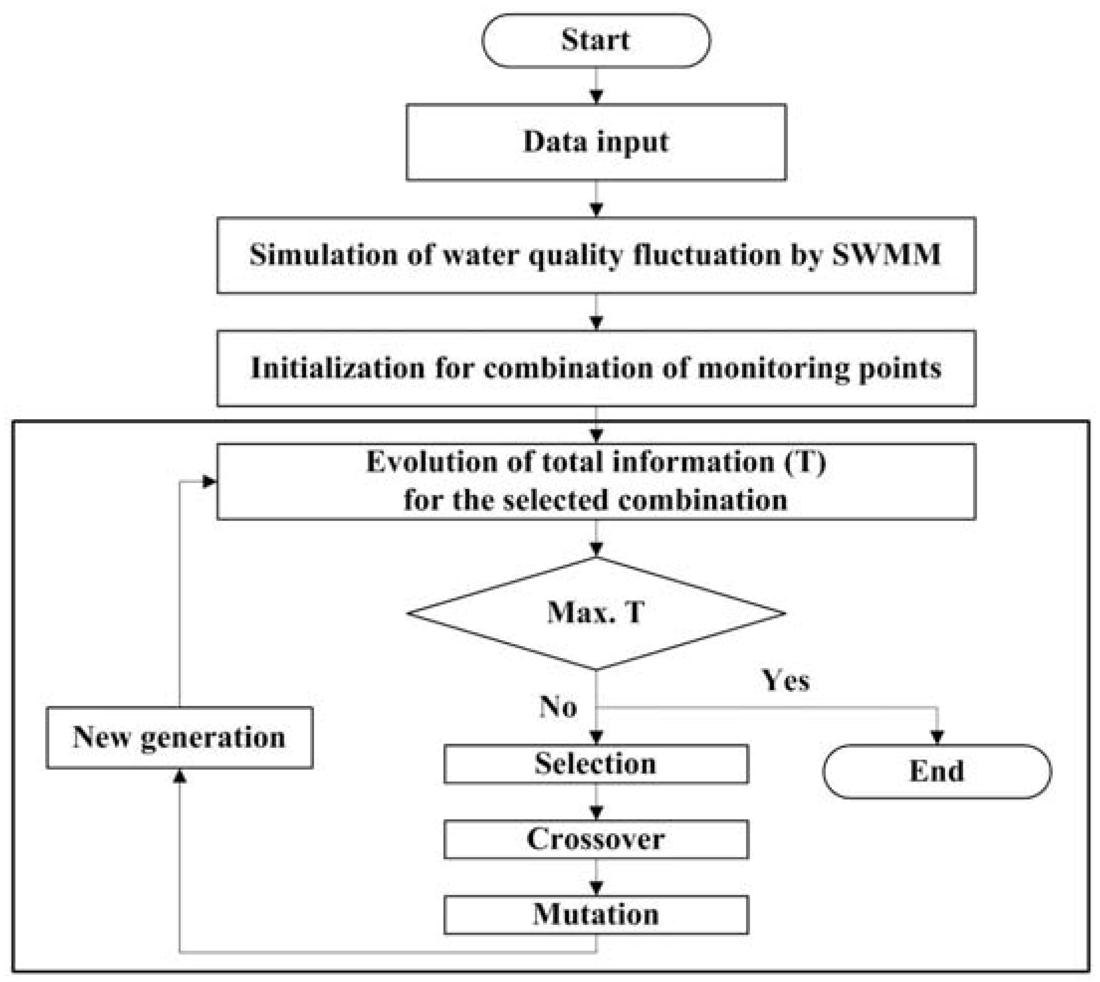
To solve the objective function, a genetic algorithm (GA) was used in this study. A GA is a heuristic search method based on the modeling of the Darwinian competition for the survival of the fittest [
28]. To obtain the optimal solution, a population of potential solutions is maintained during several cycles of circulation and each solution is evaluated based on objective function values to provide the standard for the goodness of fit. In the process, dominant entities are selected to form a new population. Some entities of the new population undergo evolution by cross-fertilization and mutation to produce a new solution. Because the GA looks for the optimal solution from all possible combinations, it rarely ends in a local optimum, unlike existing nonlinear problem search methods.
Table 1.
Selection of parameters [
27].
Table 1.
Selection of parameters [27].
| | |
| Land use | D | | | | |
| | | | | | | |
| High density residential land use | >5 | −0.0173 | 1.9456 | −0.0114 | 1.7599 | −0.0157 | 2.8651 | −72.680 | 6199.2 |
The entropy measures were calculated based on the simulation results of SWMM and the fitness of these measures is assessed by a GA. Coupling SWMM and the GA provides the framework for the optimization model for the selection of water quality monitoring points (
Figure 1).
Figure 1.
Model for the selection of the water quality monitoring points.
Figure 1.
Model for the selection of the water quality monitoring points.
4. Applications and Results
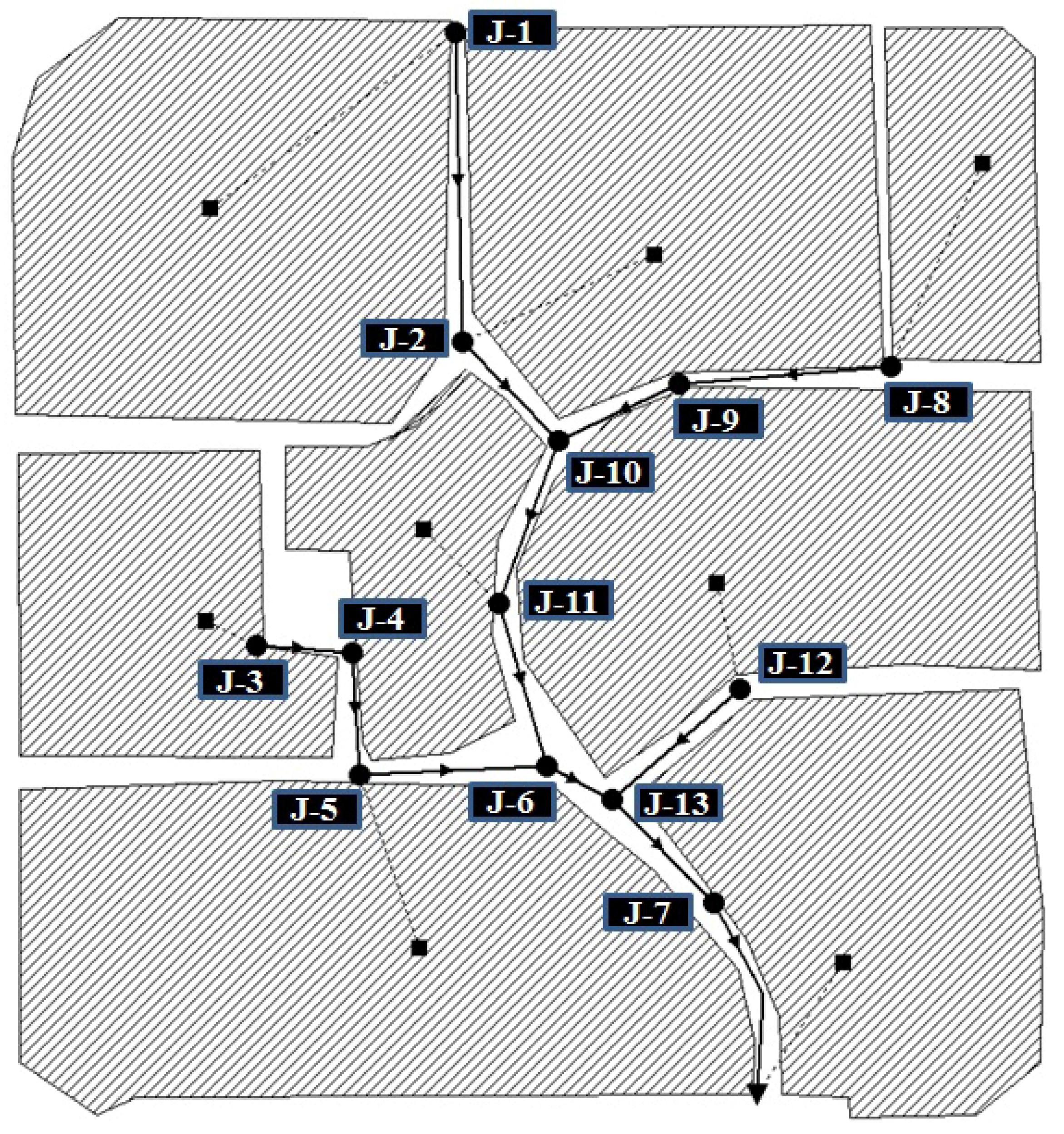
The proposed model was applied to both an example sewer network and a larger real sewer network. The example network comprises 13 manhole junctions with a drainage area of 28.7 ha, which can be divided into eight sub-basins (
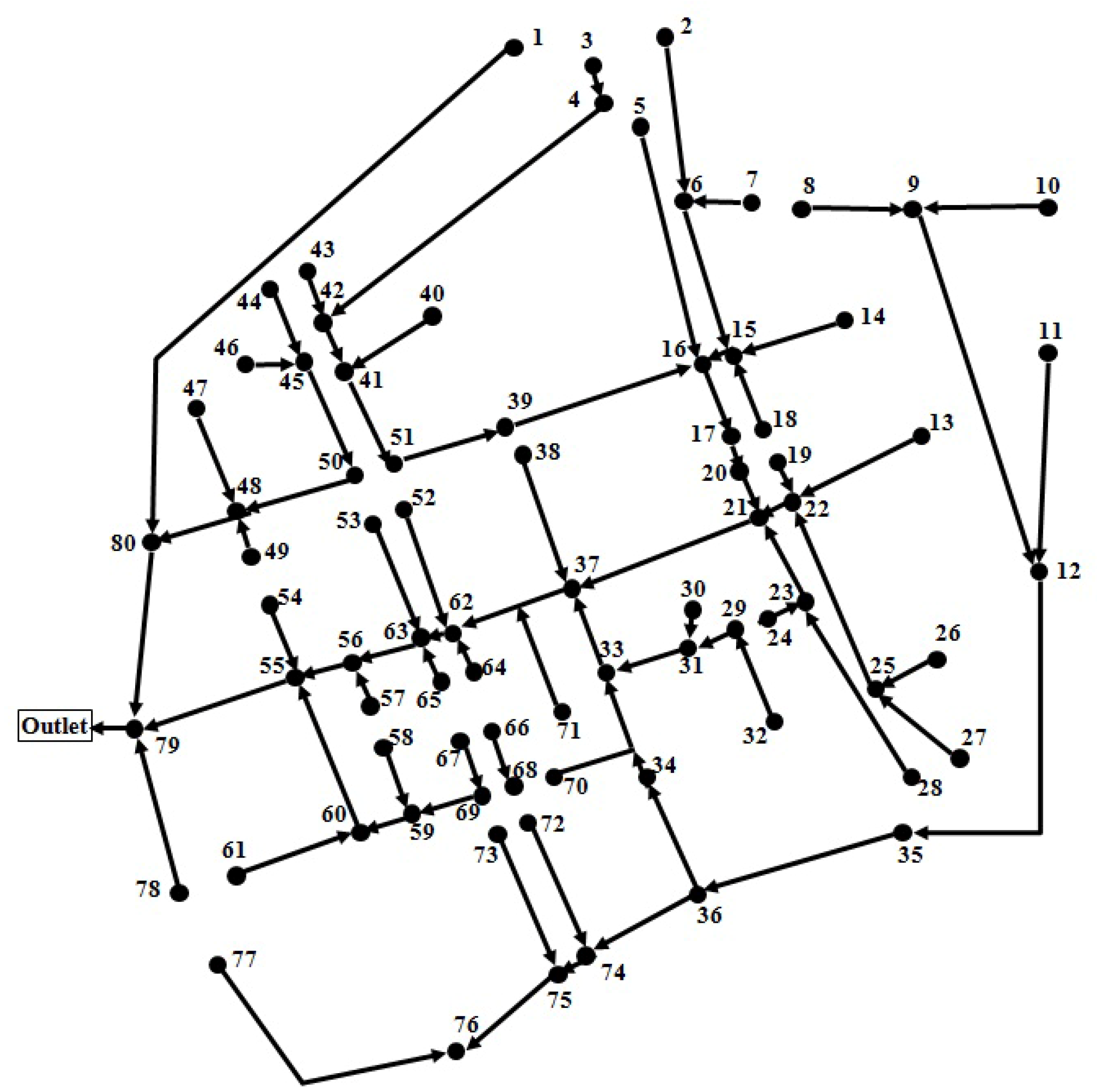
Figure 2). The real sewer network is that for the Hagye basin located in Seoul (
Figure 3). The basin has an area of 161 ha and 80 junctions where facilities of the water quality monitoring network can be installed. The used rainfall data were for the period 2002 to 2011. When SWMM was carried out, each rainfall event produced different TSS values for each junction. In this study, the average of the values was considered as the TSS, which represents each junction, and this value was used to estimate the optimal quality monitoring position.
Whether univariate or multivariate, entropy measures depend on the class interval size Δx. This dependence is such that for each selected value of Δx, different marginal, joint and conditional entropies are obtained [
25,
29]. However, the effects of the choice of different Δx values are negligible in computations of trans-information. Therefore, the variation of entropy measures with Δx does not significantly affect space/time design which is based on trans-information [
3]. Therefore, in this study, the class interval size Δx was fixed at 1mg/L and the entropy variates were calculated by applying Δx/x which is proportional to the scope of the variables.
Figure 2.
Example sewer network.
Figure 2.
Example sewer network.
Figure 3.
Hagye basin sewer network.
Figure 3.
Hagye basin sewer network.
To evaluate the objective function, the marginal entropy and trans-information among the given variates are generally expressed by one information matrix [
17,
19]. An information matrix of size 13 × 13 was constructed for the example network (
Table 2). An information matrix summarizes the marginal entropy of points and trans-information between two points. The gray area in
Table 2 represents the marginal entropy of the points. The total of each row or column refers to the trans-information when one position is selected from multiple positions. Therefore, these values refer to the amount of information that can be obtained when the position is selected from the positions where water quality monitoring facilities can be installed.
Different methods can be used to select the positions that satisfy the objective function that enables the acquisition of maximum quantity of information from multiple positions. Al-Zahrani and Husain [
17] used the method of successively selecting locations with the largest marginal entropy in the information matrix to select the combination with the largest amount of trans-information from the selected locations (A-H method). On the other hand, Kwon and Yoo [
19] selected the combination with the largest amount of trans-information from the selected locations by ordering the selected locations with the largest trans-information values from the multiple locations as shown in the bottom row of the table of the information matrix (K-Y method). However, neither of these methods guarantees the optimum combination for the objective function that maximizes the multi-location trans-information. Therefore, the optimization method was applied to identify the combination of locations with the maximum multi-location trans-information values.
To compare these three methods, the proposed model was applied to the example network. Since the number of water quality monitoring points also has to be determined, the three above methods were tested for cases with a number of monitoring points ranging from 1 to 13 (
Table 3). For all three methods, the objective function value
gradually increased with increasing number of monitoring positions, but then decreased after a certain threshold of between eight and 10 positions, depending on the method. This revealed the optimal number of monitoring positions for maximizing
(colored gray in
Table 3), beyond which any further increase in the number of monitoring positions is ineffective.
Comparing results for the optimal number of monitoring positions from the three methods tested here,
of the optimization method is greater than those of the other methods. This indicates that the optimization method is likely to be the best choice. With these preliminary results obtained for the example network, the Hagye basin (
Table 4) was investigated for which the three methods were again compared (
Table 5). Again the optimization method was verified to be superior to the A-H and K-Y methods, as it maximized the
.
These results verified that the optimization method is the best in obtaining the maximum trans-information value among the three methods tested in this study.
Table 5 shows the best combination of monitoring points selected by the optimization method. In practice, however, it is difficult to monitor at the all optimal points because of budget limits. Therefore, the optimization algorithm was applied again to optimally select water quality monitoring points within the budget limit. For example,
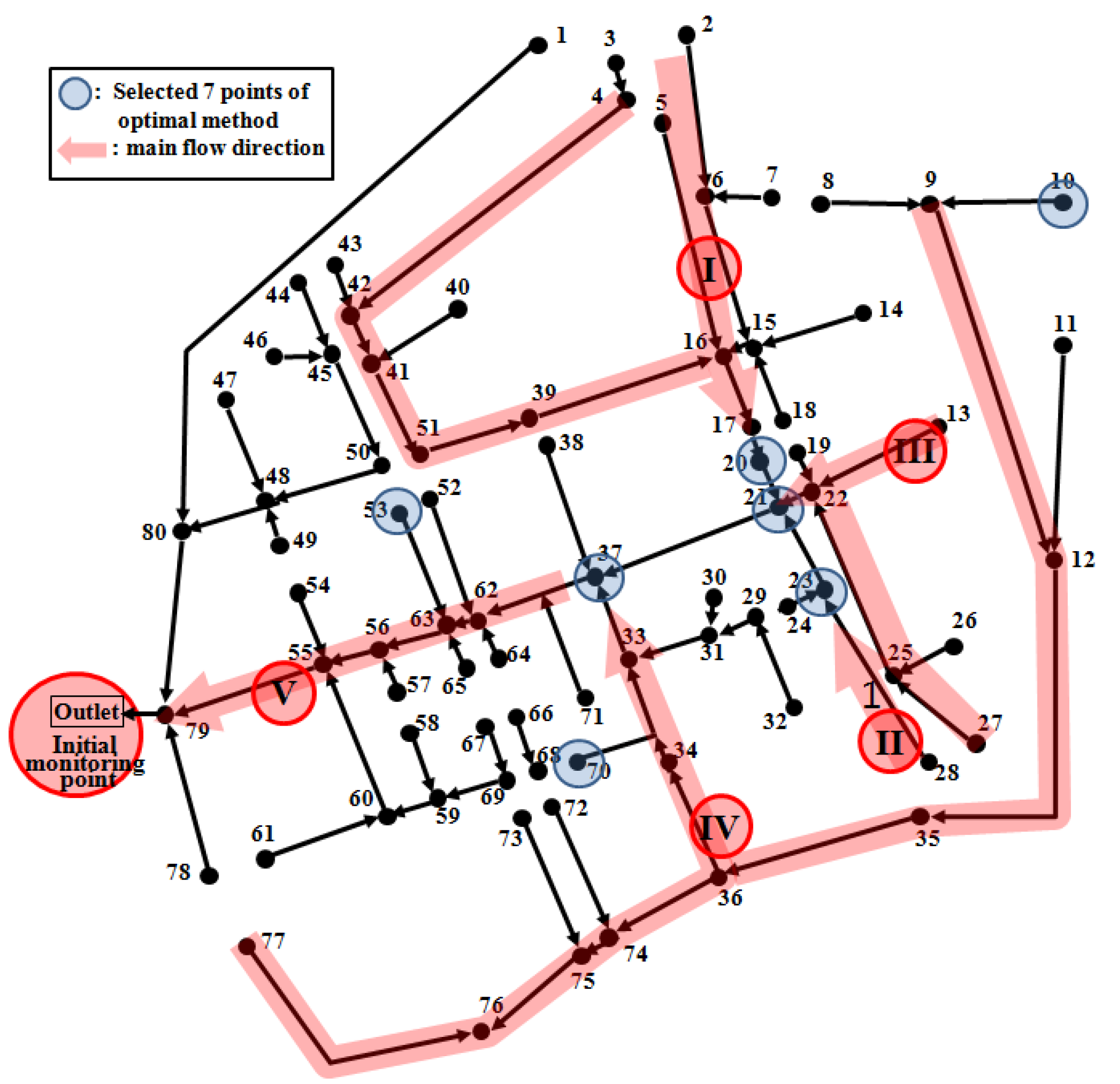
Table 6 shows the optimum combination of monitoring points when the monitoring points were limited to seven points. The locations of these seven points are shown in
Figure 4.
Table 2.
Information matrix of the example network.
Table 2.
Information matrix of the example network.
| Junction |
| 1 | 2 | 3 | 4 | 5 | 6 | 7 | 8 | 9 | 10 | 11 | 12 | 13 |
| Junction | 1 | 4.243 | 0.953 | 1.151 | 1.195 | 1.343 | 1.222 | 0.517 | 0.869 | 0.839 | 0.902 | 0.377 | 0.402 | 0.246 |
| 2 | 0.953 | 3.767 | 0.713 | 0.738 | 0.914 | 1.170 | 0.463 | 0.653 | 0.639 | 1.006 | 0.411 | 0.306 | 0.221 |
| 3 | 1.151 | 0.713 | 4.334 | 1.355 | 1.168 | 0.957 | 0.405 | 0.843 | 0.799 | 0.657 | 0.286 | 0.370 | 0.191 |
| 4 | 1.195 | 0.738 | 1.355 | 4.310 | 1.214 | 0.993 | 0.429 | 0.863 | 0.822 | 0.696 | 0.302 | 0.384 | 0.203 |
| 5 | 1.343 | 0.914 | 1.168 | 1.214 | 4.197 | 1.198 | 0.546 | 0.901 | 0.875 | 0.903 | 0.366 | 0.411 | 0.249 |
| 6 | 1.222 | 1.170 | 0.957 | 0.993 | 1.198 | 3.845 | 0.559 | 0.873 | 0.849 | 1.018 | 0.395 | 0.388 | 0.251 |
| 7 | 0.517 | 0.463 | 0.405 | 0.429 | 0.546 | 0.559 | 3.448 | 0.639 | 0.701 | 0.666 | 0.369 | 0.577 | 0.509 |
| 8 | 0.869 | 0.653 | 0.843 | 0.863 | 0.901 | 0.873 | 0.639 | 2.995 | 1.321 | 0.702 | 0.295 | 0.534 | 0.263 |
| 9 | 0.839 | 0.639 | 0.799 | 0.822 | 0.875 | 0.849 | 0.701 | 1.321 | 2.992 | 0.730 | 0.312 | 0.575 | 0.290 |
| 10 | 0.902 | 1.006 | 0.657 | 0.696 | 0.903 | 1.018 | 0.666 | 0.702 | 0.730 | 3.593 | 0.496 | 0.405 | 0.311 |
| 11 | 0.377 | 0.411 | 0.286 | 0.302 | 0.366 | 0.395 | 0.369 | 0.295 | 0.312 | 0.496 | 3.648 | 0.620 | 0.752 |
| 12 | 0.402 | 0.306 | 0.370 | 0.384 | 0.411 | 0.388 | 0.577 | 0.534 | 0.575 | 0.405 | 0.620 | 2.837 | 0.842 |
| 13 | 0.246 | 0.221 | 0.191 | 0.203 | 0.249 | 0.251 | 0.509 | 0.263 | 0.290 | 0.311 | 0.752 | 0.842 | 3.476 |
| Marginal entropy | Value | 4.243 | 3.767 | 4.334 | 4.310 | 4.197 | 3.845 | 3.448 | 2.995 | 2.992 | 3.593 | 3.648 | 2.837 | 3.476 |
| Rank | 3 | 6 | 1 | 2 | 4 | 5 | 10 | 11 | 12 | 8 | 7 | 13 | 9 |
| Trans-information | Value | 14.258 | 11.953 | 13.228 | 13.506 | 14.286 | 13.720 | 9.828 | 11.751 | 11.744 | 12.086 | 8.629 | 8.651 | 7.804 |
| Rank | 2 | 7 | 5 | 4 | 1 | 3 | 10 | 8 | 9 | 6 | 12 | 11 | 13 |
Table 3.
Monitoring points selected by three methods for the example network.
Table 3.
Monitoring points selected by three methods for the example network.
| Number of monitoring positions | Selected junctions | |
|---|
| A-H method | K-Y method | Optimization method | A-H method | K-Y method | Optimization method |
|---|
| 1 | 3 | 5 | 5 | 13.228 | 14.286 | 14.286 |
| 2 | 3,4 | 1,5 | 1,5 | 24.024 | 25.858 | 25.858 |
| 3 | 1,3,4 | 1,5,6 | 1,5,6 | 33.591 | 34.737 | 34.737 |
| 4 | 1,3,4,5 | 1,4,5,6 | 1,4,5,6 | 40.426 | 41.630 | 41.630 |
| 5 | 1,3,4,5,6 | 1,3,4,5,6 | 1,3,5,10,13 | 45.405 | 45.405 | 47.419 |
| 6 | 1,2,3,4,5,6 | 1,3,4,5,6,10 | 1,3,5,6,7,11 | 48.382 | 49.137 | 52.231 |
| 7 | 1,2,3,4,5,6,11 | 1,2,3,4,5,6,10 | 1,2,3,5,9,11,13 | 52.739 | 50.103 | 55.714 |
| 8 | 1,2,3,4,5,6,10,11 | 1,2,3,4,5,6,8,10 | 1,2,3,4,7,9,11,13 | 53.467 | 53.467 | 58.573 |
| 9 | 1,2,3,4,5,6,10,11,13 | 1,2,3,4,5,6,8,9, 10 | 1,2,3,4,7,8,10,11,13 | 56.422 | 48.442 | 59.749 |
| 10 | 1,2,3,4,5,6,7,10,11,13 | 1,2,3,4,5,6,7,8,9,10 | 1,2,3,4,7,8,10,11,12,13 | 57.323 | 48.420 | 59.521 |
| 11 | 1,2,3,4,5,6,7,8,10,11,13 | 1,2,3,4,5,6,7,8,9,10,12 | 1,2,3,4,5,7,8,10,11,12,13 | 55.272 | 48.366 | 57.776 |
| 12 | 1,2,3,4,5,6,7,8,9,10,11,13 | 1,2,3,4,5,6,7,8,9,10,11,12 | 1,2,3,4,5,7,8,9, 10,11,12,13 | 50.662 | 48.536 | 53.714 |
| 13 | 1,2,3,4,5,6,7,8,9,10,11,12,13 | 1,2,3,4,5,6,7,8,9,10,11,12,13 | 1,2,3,4,5,6,7,8,9,10,11,12,13 | 47.684 | 47.684 | 47.684 |
Table 4.
Information matrix of the Hagye basin.
Table 4.
Information matrix of the Hagye basin.
| Junction | 1 | 2 | 3 | 4 | … | 77 | 78 | 79 | 80 | Marginal entropy | Trans-information of each position when a position is selected |
|---|
| 1 | 2.180 | 1.021 | 0.882 | 1.026 | … | 1.074 | 0.544 | 1.040 | 1.051 | 2.180 | 79.324 |
| 2 | 1.021 | 2.970 | 0.937 | 1.163 | … | 1.043 | 0.605 | 1.159 | 1.112 | 2.970 | 83.475 |
| 3 | 0.882 | 0.937 | 3.332 | 0.925 | … | 0.984 | 0.910 | 0.957 | 0.992 | 3.332 | 82.041 |
| 4 | 1.026 | 1.163 | 0.925 | 2.977 | … | 1.045 | 0.592 | 1.159 | 1.113 | 2.977 | 83.258 |
| … | … | … | … | … | … | … | … | … | … | … | … |
| 77 | 1.074 | 1.043 | 0.984 | 1.045 | … | 2.942 | 0.617 | 1.077 | 1.137 | 2.942 | 86.554 |
| 78 | 0.544 | 0.605 | 0.910 | 0.592 | … | 0.617 | 3.703 | 0.614 | 0.629 | 3.703 | 87.584 |
| 79 | 1.040 | 1.159 | 0.957 | 1.159 | … | 1.077 | 0.614 | 3.201 | 1.133 | 3.201 | 85.339 |
| 80 | 1.051 | 1.112 | 0.992 | 1.113 | … | 1.137 | 0.629 | 1.133 | 3.137 | 3.137 | 87.525 |
Table 5.
The number of water quality monitoring points and the maximum trans-information.
Table 5.
The number of water quality monitoring points and the maximum trans-information.
| Selected junctions | Number of selected junctions | Maximum trans-information |
|---|
| Optimization method | 3,6,9,10,11,13,15,16,17,18,19,20,21,23,24,27,28,30,32,33,36,37,38,39,41,43,44,46,48,52,53,54,55,60,61,69,70,72,73,79,80 | 41 | 1765.465 |
| A-H method | 3,6,7,9,10,11,12,13,14,16,17,18, 19,20,21,22,23,25,27,30,31,32,33,34,35,37,46,47,48,49,50,51,52,53,54,55,56,57,62,64,70,78,79 | 43 | 1750.734 |
| K-Y method | 1,3,10,11,20,21,23,26,28,29,30,31,32,33,34,35,36,39,40,41,42,43,44,45,49,52,53,57,58,59,60,61,62,64,65,66,70,73,74,80 | 39 | 1726.845 |
Table 6.
The optimal location of seven water quality monitoring points.
Table 6.
The optimal location of seven water quality monitoring points.
| Selected seven junctions | Multi-location trans-information |
|---|
| Optimization method | 10,20,21,23,37,53,70 | 571.302 |
| A-H method | 6,12,14,19,47,54,55 | 384.807 |
| K-Y method | 10,20,21,23,31,53,70 | 571.199 |
Figure 4.
Seven optimal monitoring points.
Figure 4.
Seven optimal monitoring points.
In sewer networks, the outlet point is selected as basic monitoring point in general. This study selected additional monitoring points for the remaining 80 points, with the outlet point fixed as initial monitoring point. The point 20 and point 23 collect the water quality characteristics of the main flow directions I and II respectively. The point 21 collects the water quality characteristics in a combined flow of the main flow directions I, II and III. In addition, the point 37 collects the water quality characteristics in a combined flow of the flow direction at the point 21 and the main flow direction IV, and finally the outlet (initial monitoring point) collects the water quality characteristics of the overall flow. Therefore, the selected monitoring points can evaluate the water quality characteristics before and after the combination of major flows. The points 10, 53 and 70 are located at major starting points on the network. However, the seven points quantitatively evaluated by entropy show a concentrated pattern at the center without being dispersed spatially on the network. Accordingly, the decision maker needs to analyze the difference in entropy values by adjusting the number of monitoring points and select the spatially dispersed monitoring points within the range of proper entropy values by considering the difference of entropy value depending on the number of monitoring points. The method proposed by this study will be able to help this procedure of the decision maker.
5. Conclusions
Entropy theory was used to propose quantified standards for selecting water quality monitoring points in a sewer system. In addition, the optimization method was introduced to establish the combination for which the multi-location, maximum trans-information value can most faithfully reflect changes of water quality in the sewer system. The application of this proposed model for the exploration of optimum solutions to an urban basin revealed its superior cost-effectiveness in comparison with two other methods. As the number of water quality monitoring points usually has to be limited because of budget restrictions, the proposed model for selecting water quality monitoring points can be used to design the optimal water quality monitoring network that maximizes the collection of efficient data from a limited number of points. In conclusion, the findings of this research can be applied to the establishment of more efficient systems of continuous sewer management and water quality monitoring in urban basins.
For the sewer networks that had not been dealt with by the previous studies, this study suggested a new analysis procedure using entropy and an optimization technique to select optimal monitoring points. However, the effects of the choice of different Δx values could not be analyzed in detail by this study. It is necessary to study a proper Δx in analyzing the entropy values of various water quality items in sewer networks through a future study. In addition, Kwon and Yoo [
19] showed a result that the results of monitoring point selection by water quality items in a river network didn’t coincide with each other. This is because the influence factor and aspect may differ from each other by water quality items. Also in this study, because of the relative difference in the result values by water quality items calculated by SWMM, the optimal set of monitoring points will vary if other water quality items are evaluated instead of TSS. When the entropy values at each point differ by water quality items, to consider various water quality items complexly, there may be a method of giving each different weight by water quality items and making it a function and a method of using the Distance Measure Method (DMM), for which it is necessary to carry out a study later.

