Optimization of Curvilinear Tracing Applied to Solar Physics and Biophysics


Abstract
:1. Introduction
2. Description of the Automated Tracing Code
- (1)
- Background suppression: The median, , of an intensity image, , is computed, and the low intensity values with are set to the base value, , with being a selectable control parameter, with a default value, , if applied, and , if ignored, while a range of 1≲ qmed ≲ 2.5 was found to be useful for noisy data. The median value, zmed, is a good estimate of the background (if the features of interest cover less than 50% of the image area) and can manually be adjusted with the multiplier, qmed, otherwise. The parts of the original image that have intensities below this base level are then rendered with a constant value, are noise-free and will automatically suppress any structure detection in the background below this base level. This new method is more flexible and efficient in suppressing faint background structures.
- (2)
- Highpass and lowpass filtering: A lowpass filter with a boxcar smoothing constant, , smooths out the data noise (e.g., photon noise with Poisson statistics in astrophysical and microscopy images; e.g., see [8]), while a highpass filter with a boxcar smoothing constant, , enhances the fine structure. The two combined filters represent a bandpass filter (with ), defined by:For theoretical and experimental reasons, a filter combination of yields the sharpest enhancement of the intermediate spatial scale and, thus, warrants optimum performance in tracing of curvilinear structures.
- (3)
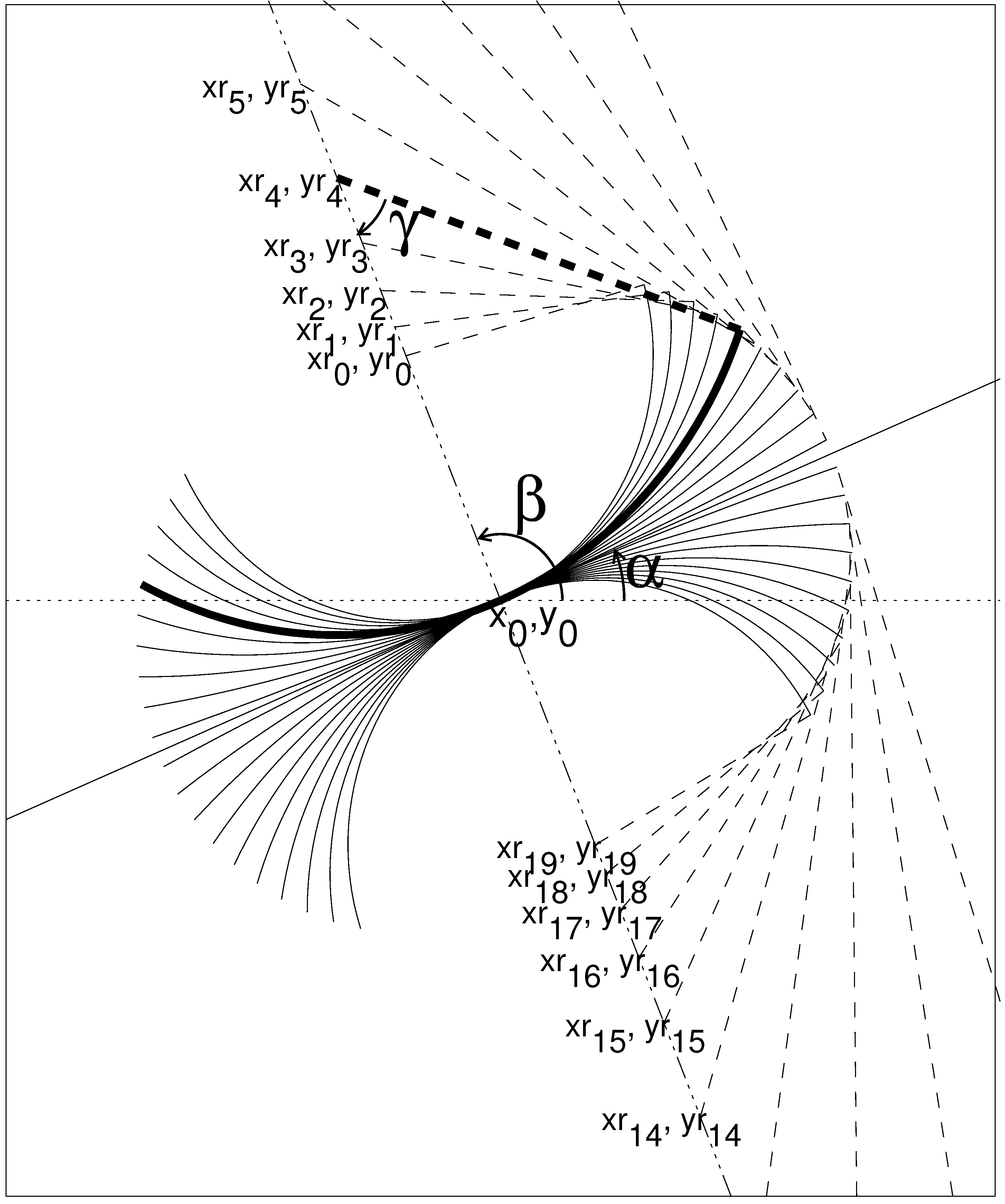
- Initialization of loop structures: The code initializes the first structure to be traced from the position, , with the maximum brightness or flux intensity, , in the original image, . Once the full loop has been traced, the area of the detected loop is erased to zero, and the next loop structure is initialized at the position, , with the next flux maximum, , in the residual image. The initialization of subsequent loops, , is continued iteratively, until the residual image becomes entirely zeroed out, the increase of detected structures stagnates or a maximum loop number, , is reached.
- (4)
- Loop structure tracing: An initialized structure starting at its flux maximum position, , is then traced in the forward direction to the first end point of the loop and, then, in the opposite direction from the original starting point to the second endpoint. The two bi-directional segments are then combined into a single uni-directional 1D path, , . The step-wise tracing along a loop structure position, , is carried out by determining, first, the direction of the local ridge (defined by the azimuthal angle, , with respect to the x-axis) and, secondly, by determining the local curvature radius, . The curved segment that follows a local ridge closest is used as a second-order polynomial to extrapolate the traced loop segment by one incremental step (of pixel). This second-order guiding criterion represents an improvement over the first-order guiding criterion used in the previous OCCULT code [7]. The second-order guiding criterion is defined by the brightness distribution, , along a loop segment with constant curvature radius and length, . If the segment follows an ideal ridge with a constant curvature radius and a constant brightness, the summed (or averaged) flux along the ridge segment has a maximum value, while it exhibits a minimum in the perpendicular direction to the ridge, where the brightness profile collapses to a δ-function.
- (5)
- Loop subtraction in residual image: Once a full loop structure has been traced, the loop area, , , is set to zero within a half width of , so that the area of a former detected loop is not used in the detection of subsequent loops. However, crossing loops can still be connected over a gap.
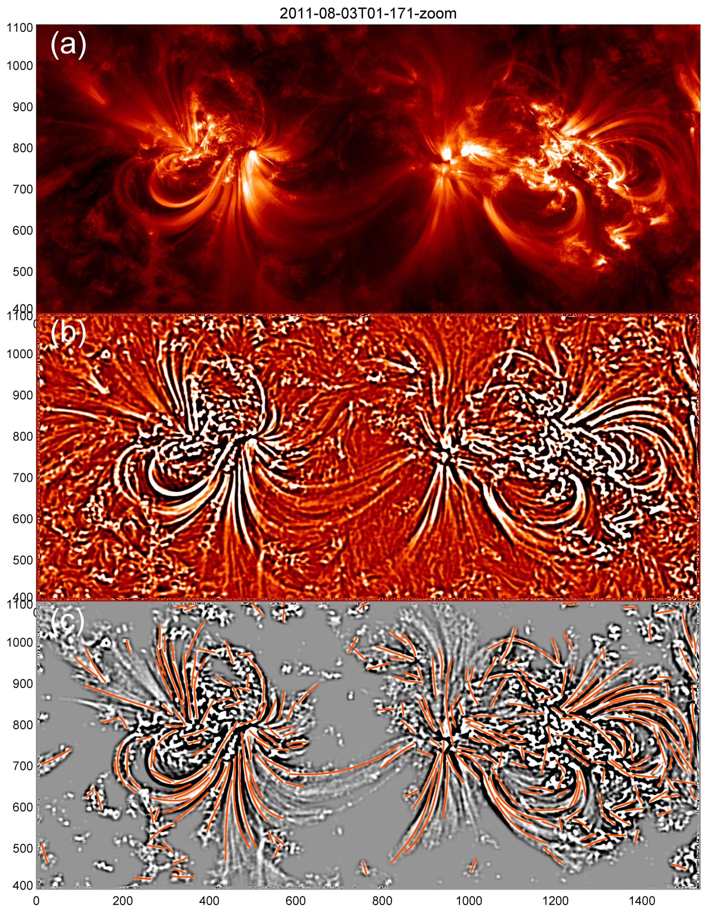
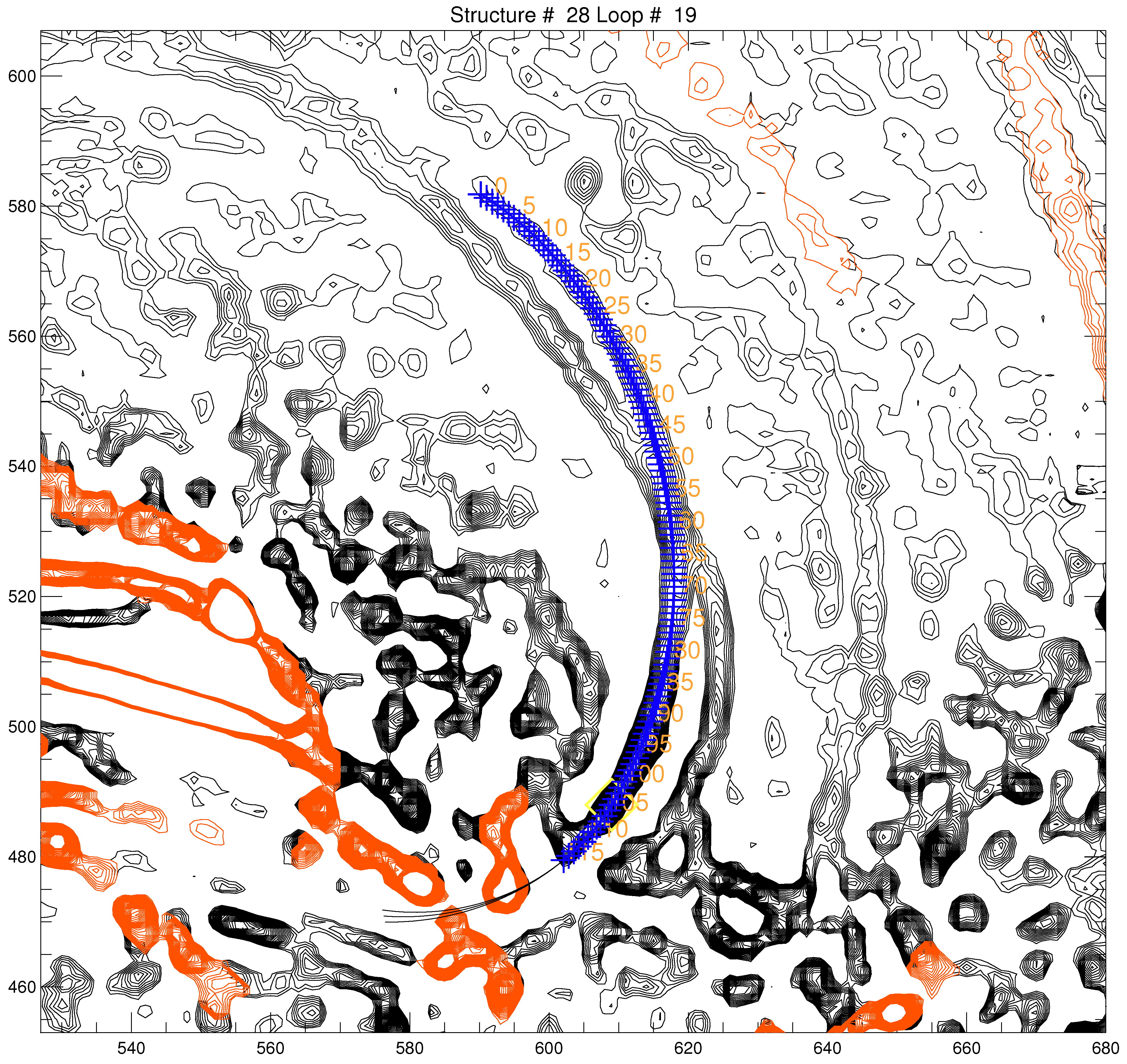
3. Application to Solar Physics

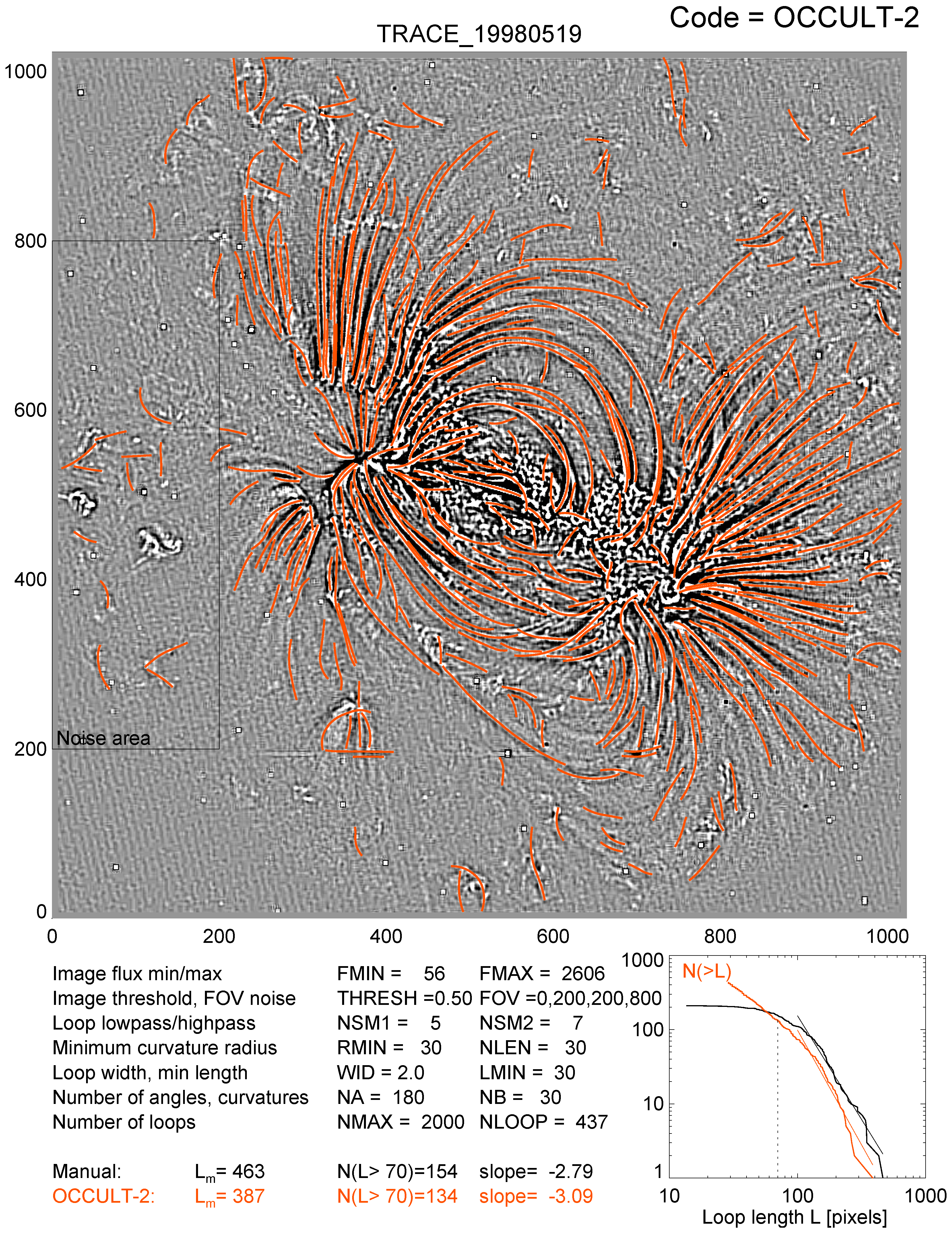
| Image | Brightness range | Minimum curvature | Filter range | Number of all loops | Number of long loops | Power-law slope |
|---|---|---|---|---|---|---|
| TRACE | 56, 2606 | 30 | 5, 7 | 437 | 134 | 3.1 |
| SDO/AIA | 28, 255 | 30 | 9, 11 | 503 | 121 | 2.7 |
| SST | 339, 916 | 30 | 3, 5 | 1757 | 376 | 3.9 |
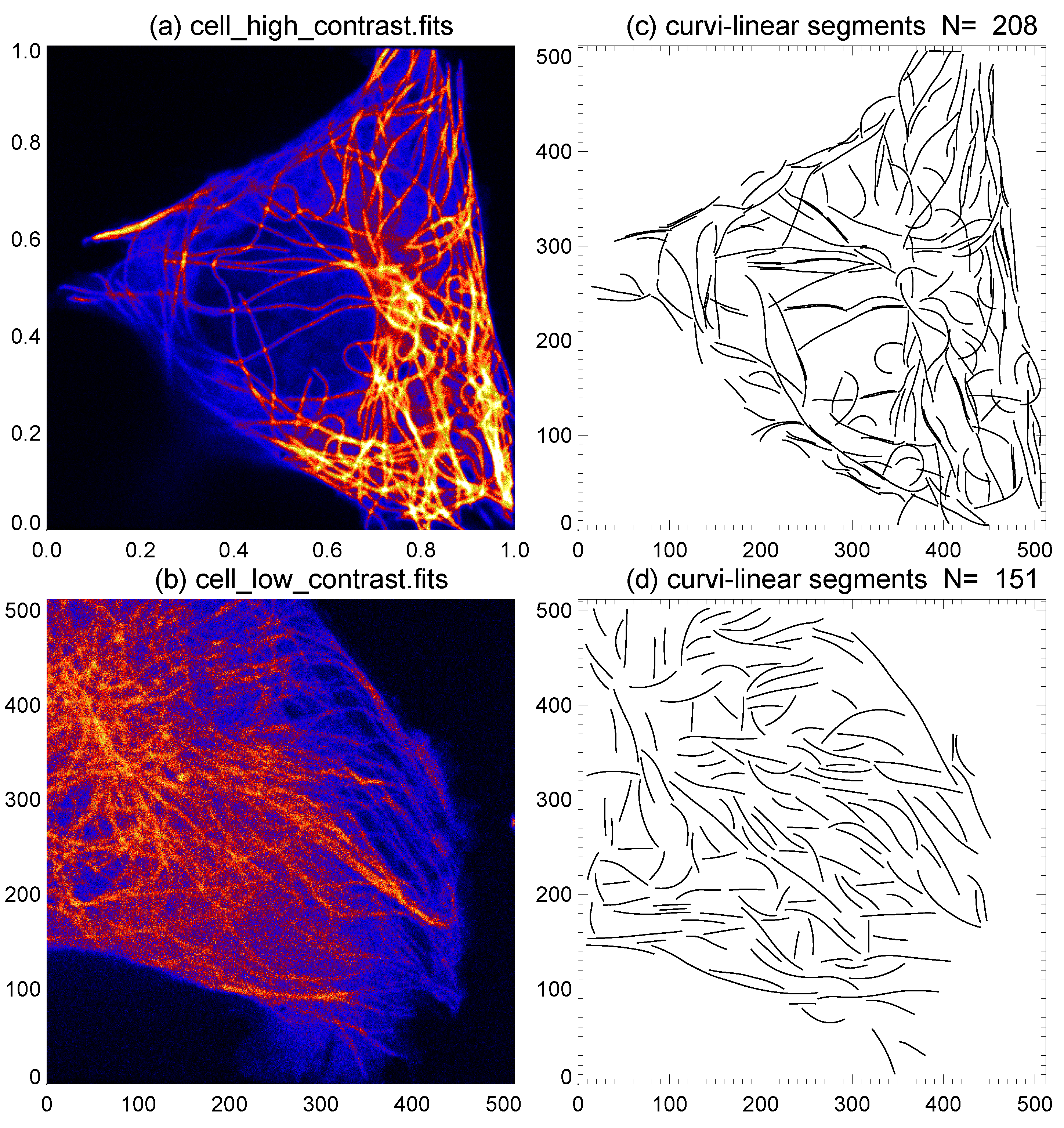
| Cell-HC | 416, 65535 | 15 | 3, 5 | 208 | 51 | 3.1 |
| Cell-LC | 289, 18699 | 30 | 7, 9 | 151 | 39 | 2.7 |
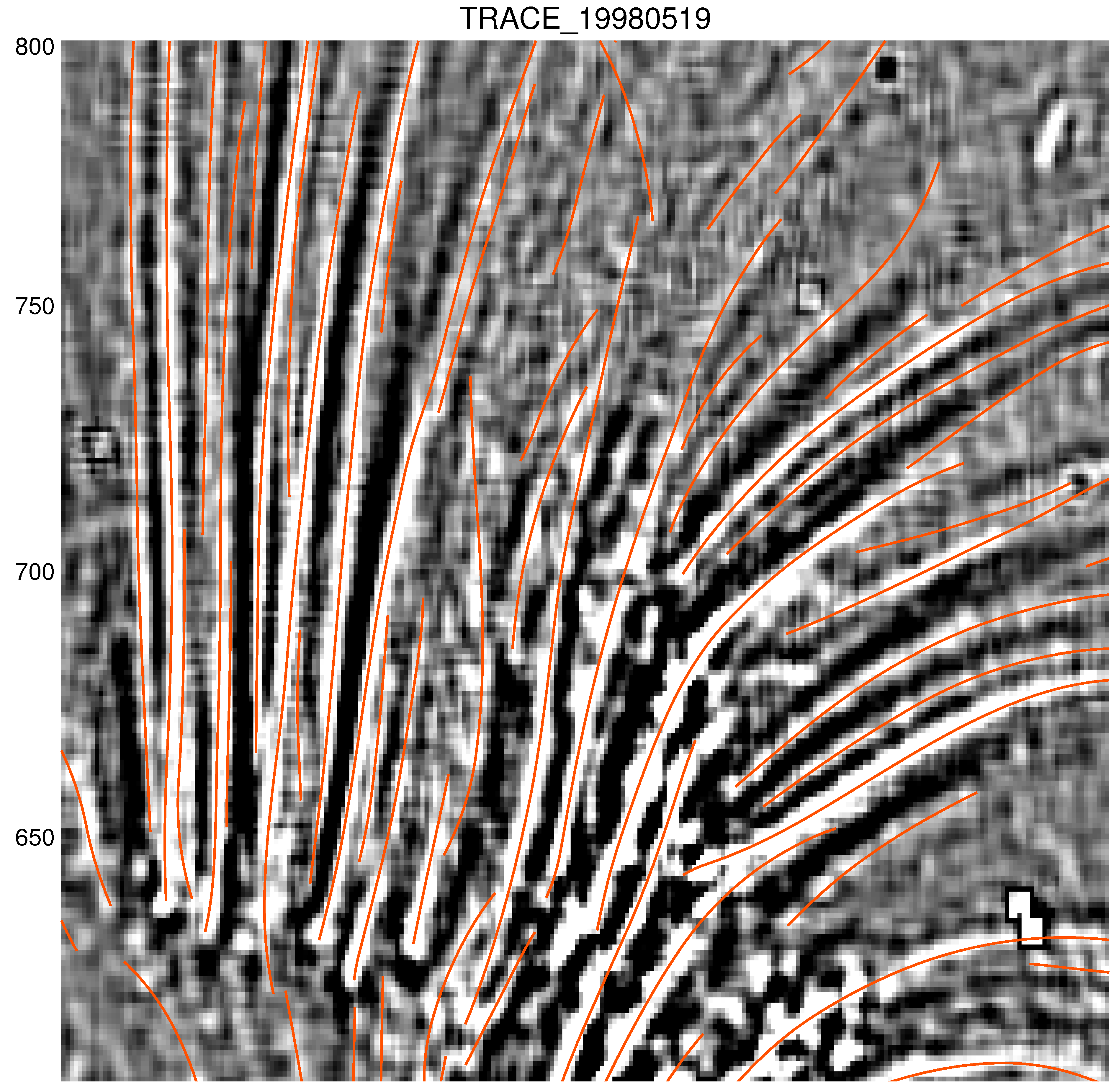
3.1. TRACE Data
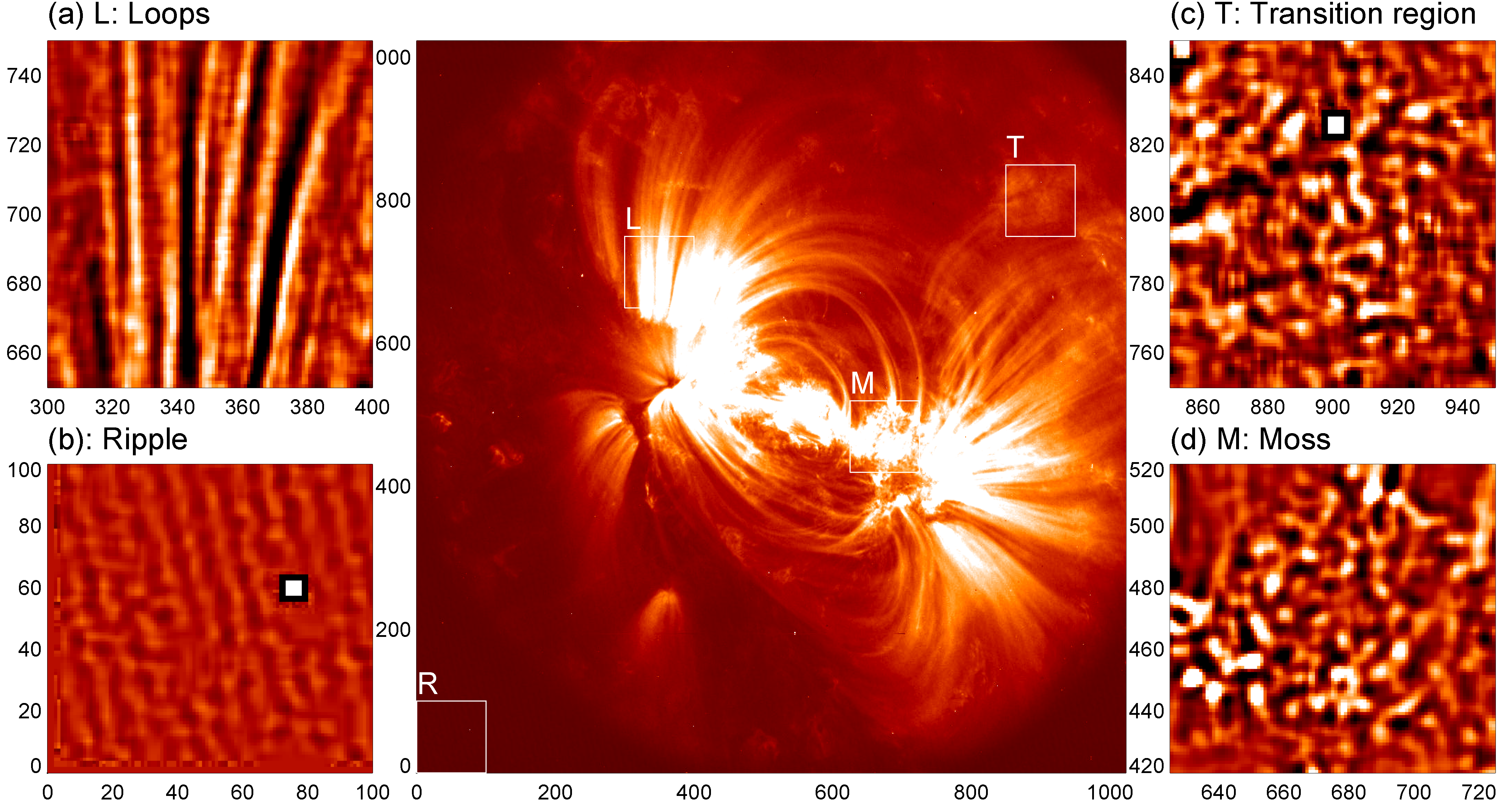
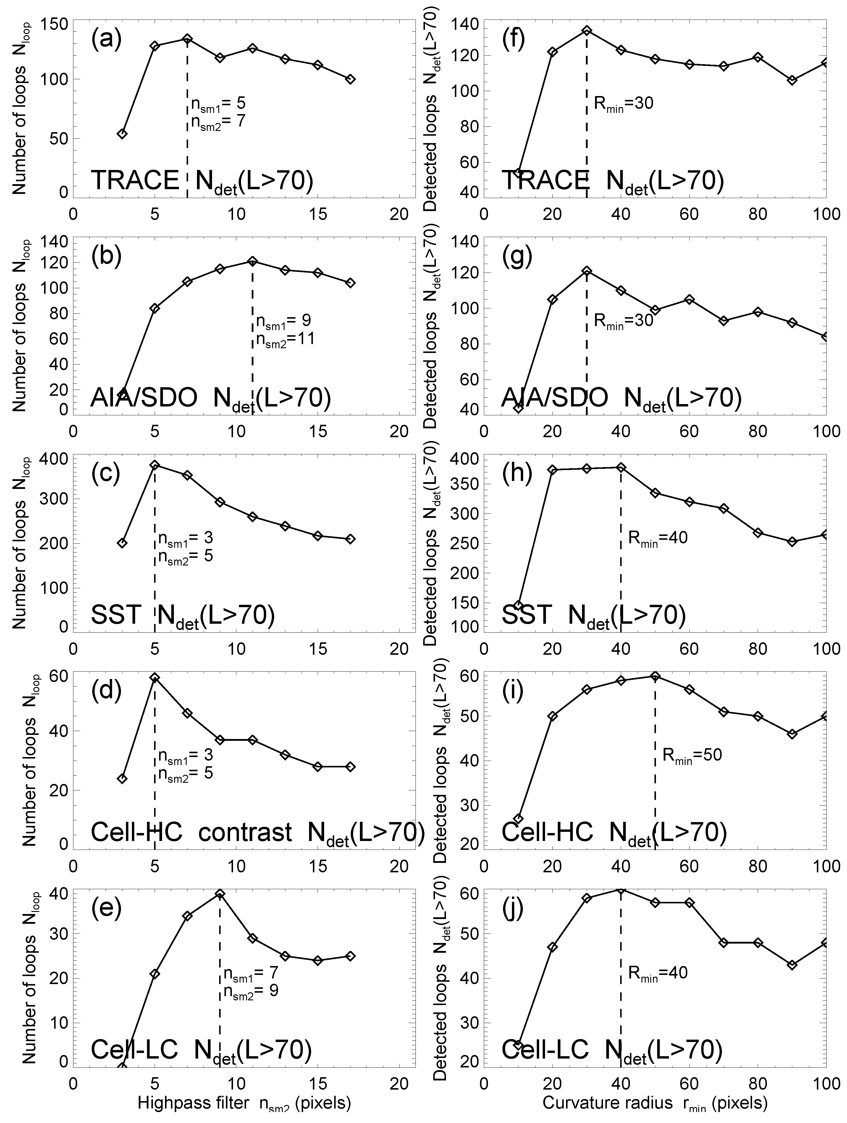
3.2. SDO/AIA Data

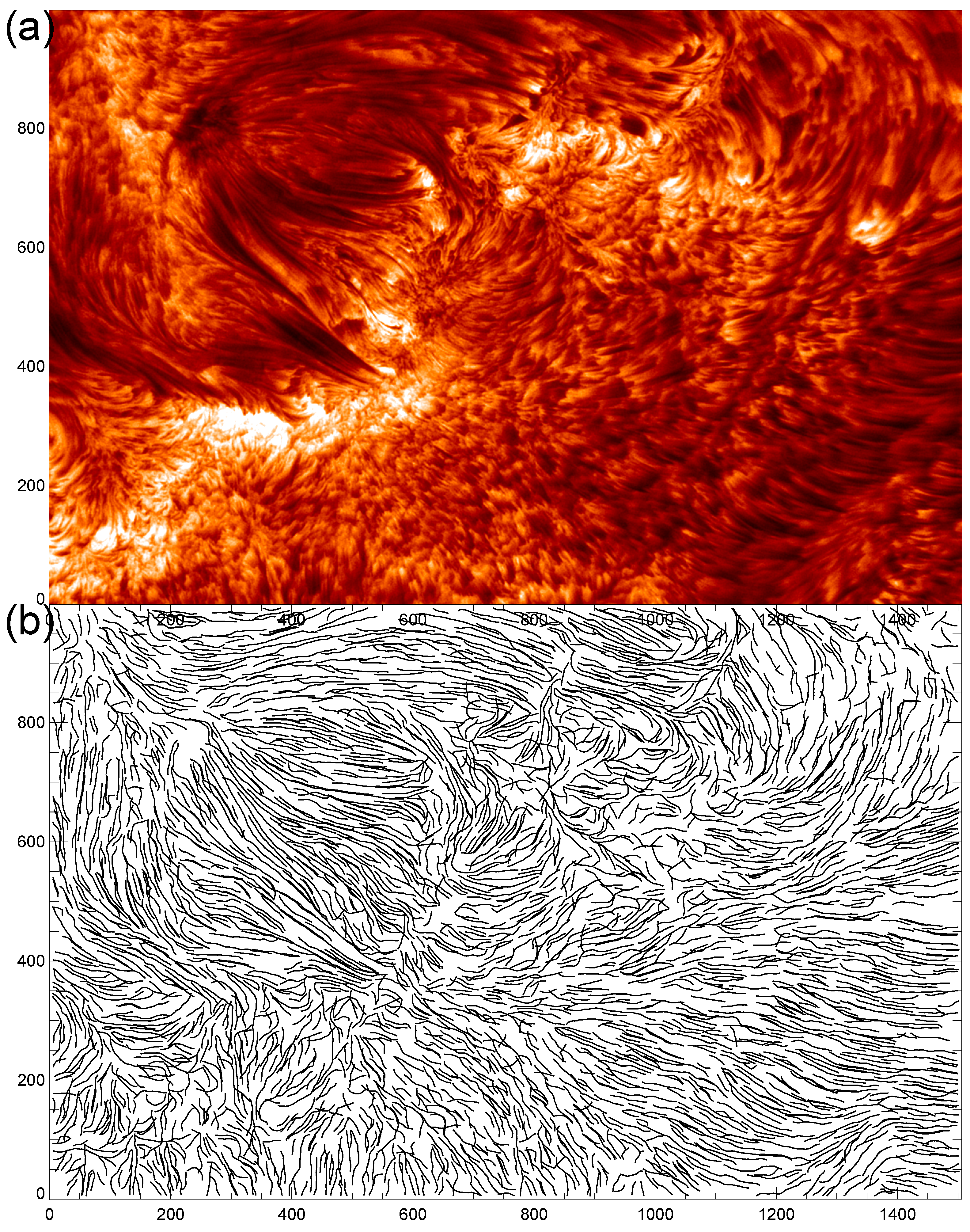
3.3. SST Data
4. Applications to Biophysics
5. Discussion and Conclusions
5.1. Optimization of Automated curvilinear Tracing
5.2. Solar Applications
5.3. Biological Applications
Acknowledgments
Conflict of Interest
References
- Gonzales, R.C.; Woods, R.E. Digital Image Processing; Pearson Prentice Hall: Upper Saddle River, NJ, USA, 2008; pp. 689–794. [Google Scholar]
- Biskri, S.; Antoine, J.-P.; Inhester, B.; Mekideche, F. Extraction of solar coronal magnetic loops with the directional 2D morlet wavelet transform. Solar Phys. 2010, 262, 373–385. [Google Scholar] [CrossRef]
- McAteer, R.T.J.; Gallagher, P.T.; Ireland, J. Statistics of active region complexity: A large-scale fractal dimension survey. Astrophys. J. 2005, 631, 628–635. [Google Scholar] [CrossRef]
- Lee, J.K.; Newman, T.S.; Gary, G.A. Automated Detection of Solar Loops by the Oriented Connectivity Method. In Proceedings of the 17th International Conference on Pattern Recognition (ICPR), Cambridge, UK, 23–26 August 2004; p. 315.
- Lee, J.K.; Newman, T.S.; Gary, G.A. Oriented connectivity-based method for segmenting solar loops. Pattern Recognit. 2006, 39, 246–259. [Google Scholar] [CrossRef]
- Aschwanden, M.J.; Lee, J.K.; Gary, G.A.; Smith, M.; Inhester, B. Comparison of five numerical codes for automated tracing of coronal loops. Solar Phys. 2008, 248, 359–377. [Google Scholar] [CrossRef]
- Aschwanden, M.J. A code for automated tracing of coronal loops approaching visual perception. Solar Phys. 2010, 262, 399–423. [Google Scholar] [CrossRef]
- Pawley, J.B.; Masters, B.R. Handbook of biological confocal microscopy. J. Biomed. Opt. 2008, 13, 029902. [Google Scholar] [CrossRef]
- Aschwanden, M.J.; Nightingale, R.W. Elementary loop structures in the solar corona analyzed from TRACE triple-filter images. Astrophys. J. 2005, 633, 499–517. [Google Scholar] [CrossRef]
- Lemen, J.R.; Title, A.M.; Akin, D.J.; Boerner, P.F.; Chou, C.; Drake, J.F.; Duncan, D.W.; Edwards, C.G.; Friedlaender, F.M.; Heyman, G.F.; et al. The Atmospheric Imaging Assembly (AIA) on the Solar Dynamics Observatory (SDO). Solar Phys. 2012, 275, 17–40. [Google Scholar] [CrossRef]
- Aschwanden, M.J. Nonlinear force-free magnetic field fitting to coronal loops with and without stereoscopy. Astrophys. J. 2013. [Google Scholar] [CrossRef]
- Aschwanden, M.J.; Sun, Y. The Active Region 11158 during the 2011 February 15 X-Class Flare: Nonlinear Force-free Magnetic Fields and Free Energies Inferred from Automated Loop Tracing. 2013. in preparation. [Google Scholar]
- Aschwanden, M.J. Available online: http://lmsal.com/∼aschwand/software/ (accessed on 23 May 2013).
- De Pontieu, B.; Erdelyi, R.; James, S.P. Solar chromospheric spicules from the leakage of photospheric oscillations and flows. Nature 2004, 430, 536–539. [Google Scholar] [CrossRef] [PubMed]
- De Pontieu, B.; Carlsson, M.; Rouppe van der Voort, L.; Löfdahl, M.; van Noort, M.; Nordlund, Å.; Scharmer, G. Rapid temporal variability of faculae: High-resolution observations and modeling. Astrophys. J. 2006, 1405–1420. [Google Scholar] [CrossRef]
- Kaverina, I.; Straube, A. Regulation of cell migration by dynamic microtubules. Semin. Cell Dev. Biol. 2011, 22, 968–974. [Google Scholar] [CrossRef] [PubMed]
- De Forges, H.; Bouissou, A.; Perez, F. Interplay between microtubule dynamics and intracellular organization. Int. J. Biochem. Cell Biol. 2012, 44, 266–274. [Google Scholar] [CrossRef] [PubMed]
- Subramaniam, R.; Kapoor, T.M. Building complexity: Insights into self-organized assembly of microtubule-based architectures. Dev. Cell 2012, 22, 874–885. [Google Scholar] [CrossRef] [PubMed]
- Tsien, R.Y. The green fluorescent protein. Annu. Rev. Biochem. 1998, 67, 506–544. [Google Scholar] [CrossRef] [PubMed]
- Wade, R.H.; Chrétien, D. Cryoelectron microscopy of microtubules. J. Struct. Biol. 1993, 110, 1–27. [Google Scholar] [CrossRef] [PubMed]
- Abbe, E. Note on the proper definition of the amplifying power of a lens or a lens-system. J. R. Microsc. Soc. 1884, 4, 348–351. [Google Scholar] [CrossRef]
- Metcalf, T.R.; Jiao, L.; Uitenbroek, H.; McClymont, A.N.; Canfield, R.C. Is the solar chromospheric magnetic field force-free? Astrophys. J. 1995, 439, 474–481. [Google Scholar] [CrossRef]
- Gary, G.A. Evaluation of a selected case of the minimum dissipative rate method for non-force-free solar magnetic field extrapolation. Solar Phys. 2009, 257, 271–286. [Google Scholar] [CrossRef]
- Fuhrmann, M.; Seehafer, N.; Valori, G.; Wiegelmann, T. A comparison of preprocessing methods for solar force-free magnetic field extrapolation. Astron. Astrophys. 2011, 526, A70. [Google Scholar] [CrossRef]
- Jiang, Y.; Bainbridge-Smith, A.; Morris, A.B. Blood Vessel Tracking in Retinal Images. In Proceedings of the Image and Vision Computing, New Zealand, 5–7 December 2007; pp. 126–131.
- Martinez-Perez, M.E.; Hughes, A.D.; Stanton, A.V.; Thom, S.A.; Barath, A.A.; Parker, K.H. Segmentation of Retinal Blood Bessels Based on the Second Directional Derivative and Region Growing. In Proceedings of the International Conference on Image Processing (ICIP 99), Kobe, Japan, 24–28 October 1999; Volume 2, pp. 173–176.
- Tang, J.; Acton, S.T. Vessel Boundary Tracking for Intravital Microscopy via Multiscale Gradient Vector Flow Snakes. In Proceedings of the IEEE International Conference on Acoustics, Speech, and Signal Processing ICASSP 04, Singapore, 17–21 May 2004; Volume 51, pp. 316–324.
- Xiong, G.; Zhou, X.; Degterev, A.; Ji, L.; Wong, S.T. Automated neurite labeling and analysis in fluorescence microscopy images. Cytom. Part A 2006, 69A, 494–505. [Google Scholar] [CrossRef] [PubMed]
- Zhang, Y.; Zhou, X.; Witt, R.M.; Sabatini, B.L.; Adjeroh, D.; Wong, S.T. Dendritic spine detection using curvilinear structure detector and Ida classifier. NeuroImage 2007, 36, 346–360. [Google Scholar] [CrossRef] [PubMed]
- Brangwynne, C.P.; Koenderingk, G.H.; Barry, E.; Dogic, Z.; MacKintosh, F.C.; Weitz, D.A. Bending dynamics of fluctuating biopolymers probed by automated high-resolution filament tracking. Biphys. J. 2007, 93, 346–359. [Google Scholar] [CrossRef] [PubMed]
- Koulgi, P.; Sargin, M.E.; Rose, K.; Manjunath, B.S. Graphical Model-based Tracing of curvilinear Structures in Bio-image Sequences. In Proceedings of the IEEE International Conference on Pattern Recognition, Istanbul, Turkey, 23–26 August 2010; pp. 2596–2599.
- Sargin, M.E.; Altinok, A.; Rose, K.; Manjunath, B.S. Tracing curvilinear Structures in Live Cell Images. In Proceedings of the IEEE International Conference on Image Processing ICIP 07, San Antonio, TX, USA, 16–19 September 2007; Volume 6, pp. 285–288.
Appendix
A.1. Analytical Description of the OCCULT-2 Code
© 2013 by the authors; licensee MDPI, Basel, Switzerland. This article is an open access article distributed under the terms and conditions of the Creative Commons Attribution license (http://creativecommons.org/licenses/by/3.0/).
Share and Cite
Aschwanden, M.J.; De Pontieu, B.; Katrukha, E.A. Optimization of Curvilinear Tracing Applied to Solar Physics and Biophysics. Entropy 2013, 15, 3007-3030. https://doi.org/10.3390/e15083007
Aschwanden MJ, De Pontieu B, Katrukha EA. Optimization of Curvilinear Tracing Applied to Solar Physics and Biophysics. Entropy. 2013; 15(8):3007-3030. https://doi.org/10.3390/e15083007
Chicago/Turabian StyleAschwanden, Markus J., Bart De Pontieu, and Eugene A. Katrukha. 2013. "Optimization of Curvilinear Tracing Applied to Solar Physics and Biophysics" Entropy 15, no. 8: 3007-3030. https://doi.org/10.3390/e15083007