Article

Statistical Analysis of Gait Maturation in Children Using Nonparametric Probability Density Function Modeling

School of Information Science and Technology, Xiamen University, 422 Si Ming South Road, Xiamen 361005, Fujian, China
*
Author to whom correspondence should be addressed.
Entropy 2013, 15(3), 753-766; https://doi.org/10.3390/e15030753
Submission received: 21 January 2013 / Revised: 19 February 2013 / Accepted: 21 February 2013 / Published: 25 February 2013

Abstract

:
Analysis of gait dynamics in children may help understand the development of neuromuscular control and maturation of locomotor function. This paper applied the nonparametric Parzen-window estimation method to establish the probability density function (PDF) models for the stride interval time series of 50 children (25 boys and 25 girls). Four statistical parameters, in terms of averaged stride interval (ASI), variation of stride interval (VSI), PDF skewness (SK), and PDF kurtosis (KU), were computed with the Parzen-window PDFs to study the maturation of stride interval in children. By analyzing the results of the children in three age groups (aged 3–5 years, 6–8 years, and 10–14 years), we summarize the key findings of the present study as follows. (1) The gait cycle duration, in terms of ASI, increases until 14 years of age. On the other hand, the gait variability, in terms of VSI, decreases rapidly until 8 years of age, and then continues to decrease at a slower rate. (2) The SK values of both the histograms and Parzen-window PDFs for all of the three age groups are positive, which indicates an imbalance in the stride interval distribution within an age group. However, such an imbalance would be meliorated when the children grow up. (3) The KU values of both the histograms and Parzen-window PDFs decrease with the body growth in children, which suggests that the musculoskeletal growth enables the children to modulate a gait cadence with ease. (4) The SK and KU results also demonstrate the superiority of the Parzen-window PDF estimation method to the Gaussian distribution modeling, for the study of gait maturation in children.

1. Introduction

Human locomotion functions are regulated by the central nervous system, and coordinated by the musculoskeletal system. The immature motor control of young children usually results in some unstable walking patterns and erratic posture [1]. Generally, an infant is able to sit upright at about 6 months after birth, begins to crawl after 9 months, and walks with immature control of posture at around 12 months [2]. When young children first learn to walk, immature motor control leads to large fluctuations from one stride interval (time from initial contact of one foot to the subsequent contact of the same foot) to another [1]. From childhood to adulthood, the stride variability would decrease due to the development of motor skills [3,4]. The early findings of Beck et al. [5] suggested that the interrelationships between temporal and distance parameters in children were fixed by the age of 4. According to Sutherland [6], the gait in young children about 4 years old will become relatively mature, with a more stable walking pattern. Nonetheless, Norlin et al. [7] studied 230 individuals from 3 to 16 years old, and reported that the gait had not become mature until 8 years old. Menkveld et al. [8] observed a group of subjects aged from 7 to 16 years, and concluded that the temporal gait patterns presented apparent maturity but still continued developing in adolescence. Recent studies [3,4,9] focused more attention on the issue whether subtle changes in gait unsteadiness and large stride-to-stride fluctuations occur in adolescents as well. Although prospective within-subject changes in children’s gait have not been fully examined yet, the discussions based on different observations have advanced the research of gait maturation [1].
During the last decade, statistical tools have been effectively used for study of the gait and postural control in neuromuscular systems. Manabe et al. [10] applied the modified pixel dilation method to analyze the static stabilometric patterns for postural instability evaluation in Parkinson’s disease and spinocerebellar ataxia. They reported that the fractal dimensions with closed eyes are significantly higher in Parkinson’s disease and spinocerebellar ataxia groups than those in the normal control group [10]. Doyle et al. [11] used the intra-class correlation coefficient models to compare the reliability of fractal dimensions with traditional measures of quiet stance center of pressure (COP) in healthy adolescents. They concluded that the fractal dimensions are more reliable than extensively used COP measures, such as range of sway, peak sway velocity, and so forth [11]. Cimolin et al. [12] computed the fractal dimensions using the box-counting method to quantify the postural strategy of patients with Prader–Willi syndrome. Their investigation indicated that the fractal dimensions, along with the time-domain and frequency-domain parameters, of patients with Prader–Willi syndrome are statistically different in comparison with those of age-matched healthy controls [12]. To study the stride-to-stride change in adolescents, Hausdorff et al. [3] applied the fractal analysis method to measure the fluctuation magnitude in the gait rhythm time series. The work of Hausdorff et al. [3] suggested that the increased variability in younger children is not due to fatigue or a change of gait speed, and the stride-to-stride variability (in terms of the coefficient of variation) is significantly different between the children in three age groups (aged 3–4 years, 6–7 years, and 11–14 years). They also found that the temporal structure and fractal properties of stride fluctuations are associated with long-range, fractal organization, and the stride-to-stride dynamics exhibit age-dependent changes in young children [3].
Analysis of gait patterns in children helps physiologists and neuroscientists understand the natural course of gait maturation, and also provides indices that can be used to distinguish between normal immature locomotor actions and movement disorders in children. As Shumway-Cook and Woollacott suggested [13], analysis of the stride dynamics may provide a potential window into the development of children’s neuromuscular control, but further quantitative studies still call for complementary computational methods to describe the gait maturation in children. The aim of the present study was to quantify the locomotor stability based on probability density functions, and describe idiosyncratic gait patterns in healthy children by means of statistical parameters [14].

2. Data Description

The gait database used in the present study was contributed by Hausdorff et al. [3], and can also be accessed via the web page of PhysioNet [15]. Fifty healthy children participants (aged 3–14 years, 25 boys and 25 girls) were recruited from the local community in Boston, MA, USA [3]. These children were categorized into three age groups: 3- to 5-year-old (14 subjects), 6- to 8-year-old (21 subjects), and 10- to 14-year-old (15 subjects). The numbers of boys and girls were similar in each age group. The children’s parents were requested to provide informed written consent, and also to describe the medical history of their children. These children were free of neurological, cardiovascular, or musculoskeletal disorders, and none of them was born prematurely [3].
According to Hausdorff et al. [3], the children subjects were instructed to walk at their normal pace around a 400 m running track for 8 min. An investigator walked slightly behind each subject during the ambulation. Two ultrathin pressure-sensitive switches [16] were placed in each subject’s right shoe (one underneath the heel of the foot and the other underneath the ball of the foot) to record the force applied to the level ground. The temporal signals were digitized by an on-board analog-to-digital converter at the sampling rate of 300 Hz with 12 bit resolution per sample, and then stored in a recorder (dimensions: 5.5 × 2 × 9 cm 3 ; weight: 0.1 kg). The recorder was worn on the ankle cuff of each foot and held in place with a wallet on the ankle. The time series of stride interval were obtained with the algorithm proposed by Hausdorff et al. [16].

3. Gait Analysis

3.1. Signal Preprocessing

Because two legs have to modulate the acceleration or deceleration behavior at the beginning or ending of walking, the walking velocity and other gait parameters are somewhat different from those in the course of walking at normal pace. In order to minimize the start-up or ending effects of walking posture, the samples of stride interval recorded in the first 60 s (1 min) and the last 5 s were excluded, which was the same as implemented in the previous study of Hausdorff et al. [3].
A median filter [17] was applied to detect the outliers that were 3 standard deviations (SDs) in amplitude greater than the median value in the time series of stride interval. According to the well-known “three-sigma rule” [18], about 99.7% of the normally distributed probability values lies within 3-SD distance from the mean, which implies the outliers only occur with a very low probability (about 0.3%). Since some outliers possessed very large values and could affect the computing of the mean over the entire time series, we used the median value instead of the mean of the corresponding time series.
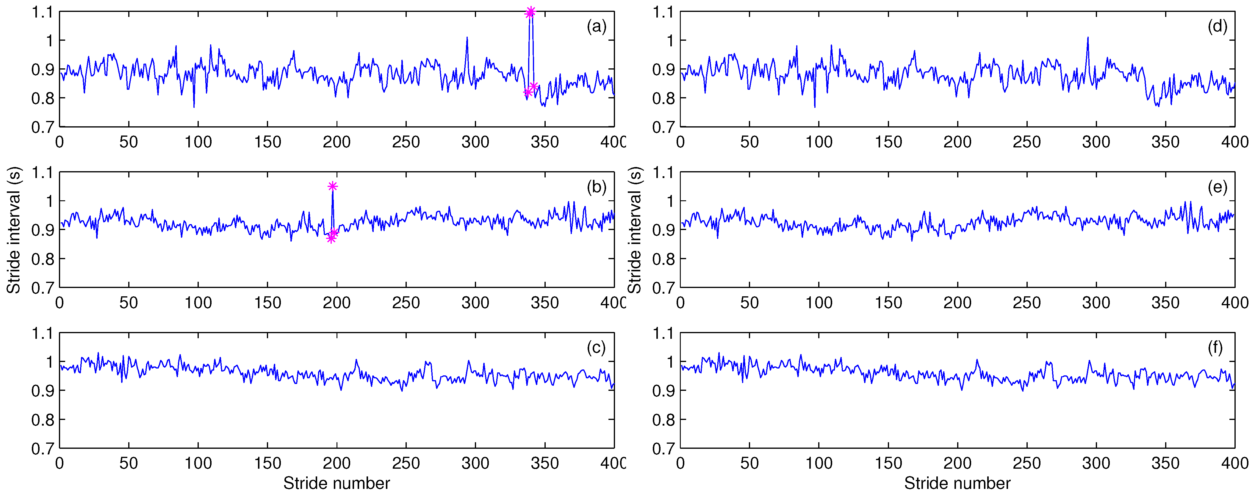
The time series examples of original and outlier-processed stride interval of the children in three different age groups are illustrated in Figure 1. Since the start-up effects have been eliminated, the first stride in each time series was made from the second minute in the 8 min monitoring. In Figure 1a and b, the outliers detected, along with one stride before or after the outliers, are marked with asterisks in the original time series. These stride interval samples, which were considered to be associated with the pauses during the gait monitoring, were removed before the gait analysis. It is noted that the child aged 129 months regulated his strides with little variation, and there is no outlier found in the time series of stride interval in Figure 1c.
Figure 1. Original time series of stride interval of the children (a) aged 45 months (in the group aged 3–5 years); (b) aged 80 months (in the group aged 6–8 years); and (c) aged 129 months (in the group aged 10–14 years), respectively. Outliers detected, along with one stride before or after the outliers, are marked with asterisks; Subfigures (d)–(f) plot the corresponding outlier-free time series of stride interval. The first strides in (a)–(f) start after the start-up 60 s (1 min).
Entropy 15 00753 g001
From Figure 1d, e and f, it is clear that these representative time series exhibit distinct characteristics. The degree of stride fluctuations is highest in the youngest child (aged 3–5 years), whereas the stride-to-stride variability of the other two children (aged 6–8 years and 10–14 years) becomes much smaller, as reported by Hausdorff et al. [3] that the stride fluctuations measured by coefficient of variation and SD of detrended time series are significant different between any two age groups ( p - value < 0.01 ). Such differences are more visible in 
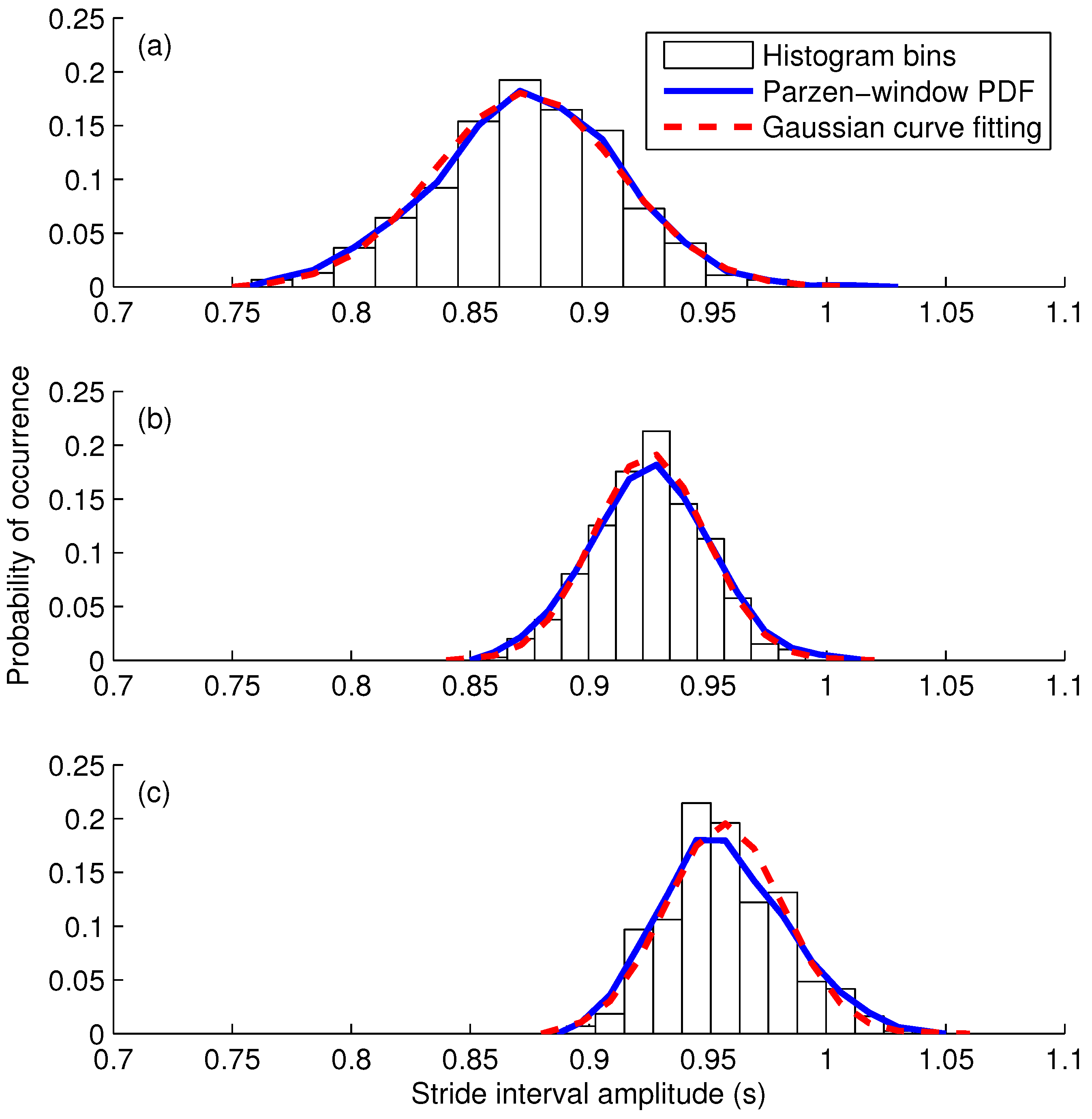
Figure 2. It can be observed that the spread of the PDF of the child aged 45 months is much wider than those of the older children aged 80 and 129 months, respectively. In addition, the mean value of the stride interval of the children aged 129 months is about 0.96 s, which is larger in amplitude than those of the younger children (0.87 and 0.93 s for aged 45 and 80 months, respectively).
Figure 2. Histograms and Parzen-window probability density functions (PDFs) estimated for the stride interval time series of the children (a) aged 45 months (in the group aged 3–5 years); (b) aged 80 months (in the group aged 6–8 years); and (c) aged 129 months (in the group aged 10–14 years), respectively.
Entropy 15 00753 g002

3.2. Probability Density Function (PDF) Estimation

In order to derive the statistical parameters related to the gait maturation in children, we first computed the histogram as a reference of PDF, for each outlier-free time series of stride interval. The histogram of stride interval can be established with B bins, which helped calculate the probability of occurrence with B containers of equal length in the amplitude range of stride interval. According to Scott’s choice [19], the optimal bin number B that helps minimize the mean squared error between the estimated histogram and the Gaussian density function can be obtained as
B = ( g m a x - g m i n ) 3.49 s n - 1 / 3
where s and n represent the SD and the number of samples in the stride interval time series, respectively; the highest and lowest values of stride interval g are denoted as g m a x and g m i n , respectively; and the operator · rounds the number of bins toward the nearest integer greater than or equal to it.
Then we applied the Parzen-window method [20] to estimate the PDF of stride interval from the outlier-free time series, for each subject. Given a M-length time series of stride interval, { g k } , k = 1 , 2 , , M , the estimated PDF p ^ ( g ) can be expressed as [14,21,22]
p ^ ( g ) = 1 M k = 1 M w g - g k
where w ( · ) is a window function that integrates to unity. In the present study, we used the popular Gaussian window function to estimate the Parzen-window PDF of stride interval, i.e.,
w ( g - g k ) = 1 σ P 2 π exp - ( g - g k ) 2 2 σ P 2
where σ P represents the spread parameter that determines the width of a Gaussian window, the center of which is located at g k [21]. In order to determine the optimal spread parameter, the Parzen-window PDF was arranged with the same resolution as the histogram, i.e., the estimated probability density, p ^ ( g b ) , b = 1 , 2 , , B , was also represented with B bins. Then the optimal spread parameter can be obtained by minimizing the mean-squared error (MSE) between the Parzen-window PDF, p ^ ( g b ) , and the histogram, h ^ ( g b ) , i.e., min 1 B b = 1 B [ p ^ ( g b ) - h ^ ( g b ) ] 2 . By searching the value of spread parameter that varied over the range from 0.001 to 0.1, with an increment of 0.001, the optimal value of σ P was set to be 0.01 in accordance with the MSE minimization criterion.
Figure 2 shows the histograms and the PDFs estimated for the representative subjects of the three age groups in Figure 1. Gaussian PDFs (dashed curves) are fit with the Gaussian distributions, the mean and variance parameters of which are equal to those of the corresponding histograms. It is worth noting that all the PDFs are unimodal, but not exactly overlap the reference Gaussian distributions. The stride interval PDF of the youngest child possesses the largest spread area, in comparison with the PDFs of the other two children. In addition, the center location of stride interval PDF seems to move toward a larger value with the increase of age. Such probability distributions motivate us to compute the statistical parameters for detailed comparisons.

3.3. Statistical Parameters

Four statistical parameters, i.e., averaged stride interval (ASI), variation of stride interval (VSI), skewness (SK), and kurtosis (KU), were computed with the Parzen-window PDF estimated [14]. The ASI and VSI represent the mean and SD values of stride interval, i.e.,
μ = b = 1 B g b p ^ ( g b )
and
σ = b = 1 B g b - μ 2 p ^ ( g b )
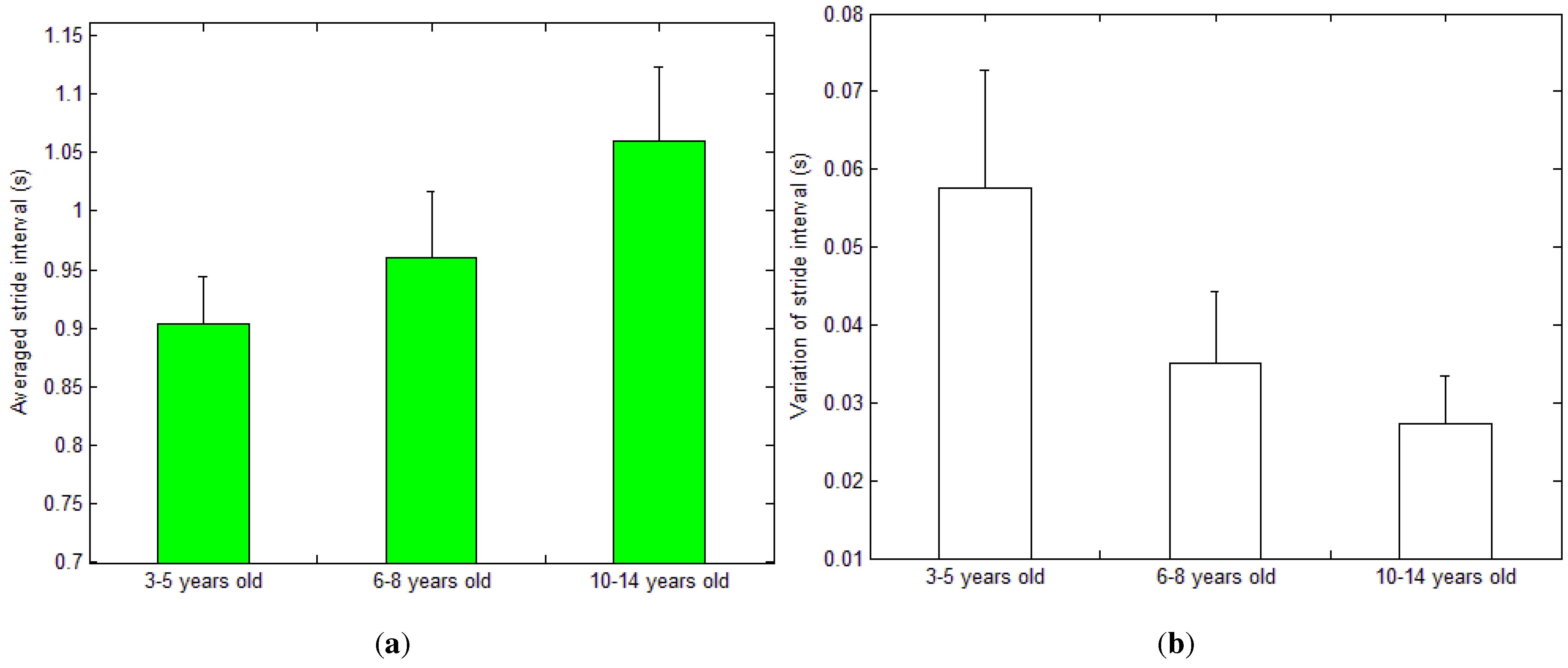
Statistical measures (ASI and VSI) of stride interval for the children in the three age groups are shown in Figure 3. The Student’s t-test [23] was also performed to test whether or not the values of the ASI and VSI are significantly different (significant level: p - value < 0 . 01 ) between any two bars for the corresponding age groups.
Figure 3. Bar graphics of (a) averaged stride interval (ASI) and (b) variation stride interval (VSI) computed from the Parzen-window probability density functions (PDFs) of the children in the groups aged 3–5 years, 6–8 years, and 10–14 years, respectively. Vertical lines on the tops of the bars denote the standard deviation (SD) values. The values (mean ± SD) of the bars for the children of 3–5 years old (ASI: 0.904 ± 0.041 s, VSI: 0.058 ± 0.015 s), of 6–8 years old (ASI: 0.96 ± 0.056 s, VSI: 0.035 ± 0.009 s), and of 10–14 years old (ASI: 1.059 ± 0.063 s, VSI: 0.027 ± 0.006 s).
Entropy 15 00753 g003
From Figure 3, we may observe that both the ASI and VSI are age-dependent: the ASI increases with age, whereas the VSI decreases when the children grow up. The ASI value for the 6- to 8-year-old age group is 0.056 s higher ( p - value < 0 . 01 ) than that for the 3- to 5-year-old age group, and the value is increased by 0.099 s ( p - value < 0 . 0001 ) comparing the 10- to 14-year-old children with that for the 6- to 8-year-old children. On the other hand, the VSI value is decreased by 0.023 s ( p - value < 0 . 0001 ) in the children aged from 3 years to 8 years, and then continues to be decreased by 0.008 s ( p - value < 0 . 001 ) until the children are 14 years old. Such results suggest that the children are more and more skilled to modulate large strides during the course of musculoskeletal growth, and the ability to control stable strides is significantly improved in the children aged 3–8 years. It can therefore be inferred that the locomotor control system in children aged 3–8 years is still rapidly developing, and will reach maturity until they are 14 years old, when their gait patterns become very close to those of healthy adults [3].
The SK and KU are two parameters that usually measure the asymmetry and “peakedness” characteristics of a PDF [24,25]. The SK and KU can be calculated from the PDF moments as
S K = m 3 ( m 2 ) 3 / 2
and
K U = m 4 ( m 2 ) 2
where m j represents the jth central moment of the PDF [26,27], defined as
m j = b = 1 B g b - μ j p ^ ( g b )
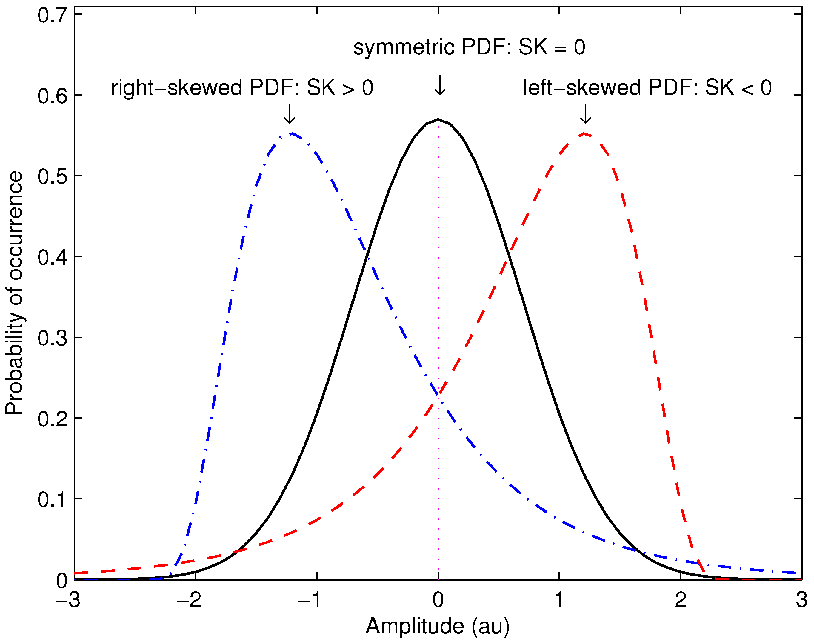
Figure 4 illustrates three typical SK values for a unimodal PDF: if the PDF is symmetric or balanced, e.g., the Gaussian distribution, the skewness is zero; if the mass of the PDF is concentrated on the left of the mean, the PDF is right-skewed, i.e., the skewness is positive (SK > 0); in contrast, if the mass of the PDF concentrates on the right of the mean, the PDF is then left-skewed, i.e., the skewness is negative (SK < 0).
Figure 4. Illustration of the probability density functions (PDFs) with three types of skewness (SK): right-skewed PDF, dash-dot curve, SK > 0 ; symmetric PDF, solid curve, SK = 0 (in particular Gaussian distributions); left-skewed PDF, dashed curve, SK < 0 . Dot line represents a central axis up to the mean of the symmetric PDF. au: arbitrary units.
Entropy 15 00753 g004
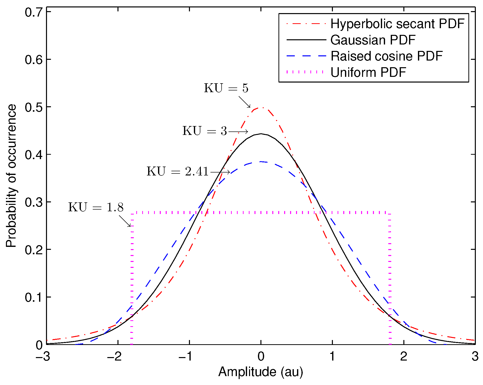
Figure 5 shows four well-known PDFs with different KU values: the sharper the peak of distribution, the larger the KU becomes. The top of uniform distribution is flat, and its KU is smallest (KU = 1.8); the Gaussian distribution possesses a KU value of 3.0, which is usually considered as the benchmark for KU comparison; the peak of the raised cosine PDF is more rounded than the Gaussian distribution, so that the KU value is 2.41; the hyperbolic secant PDF [28] has the sharpest peak and the largest KU value (KU = 5) among the four distributions.
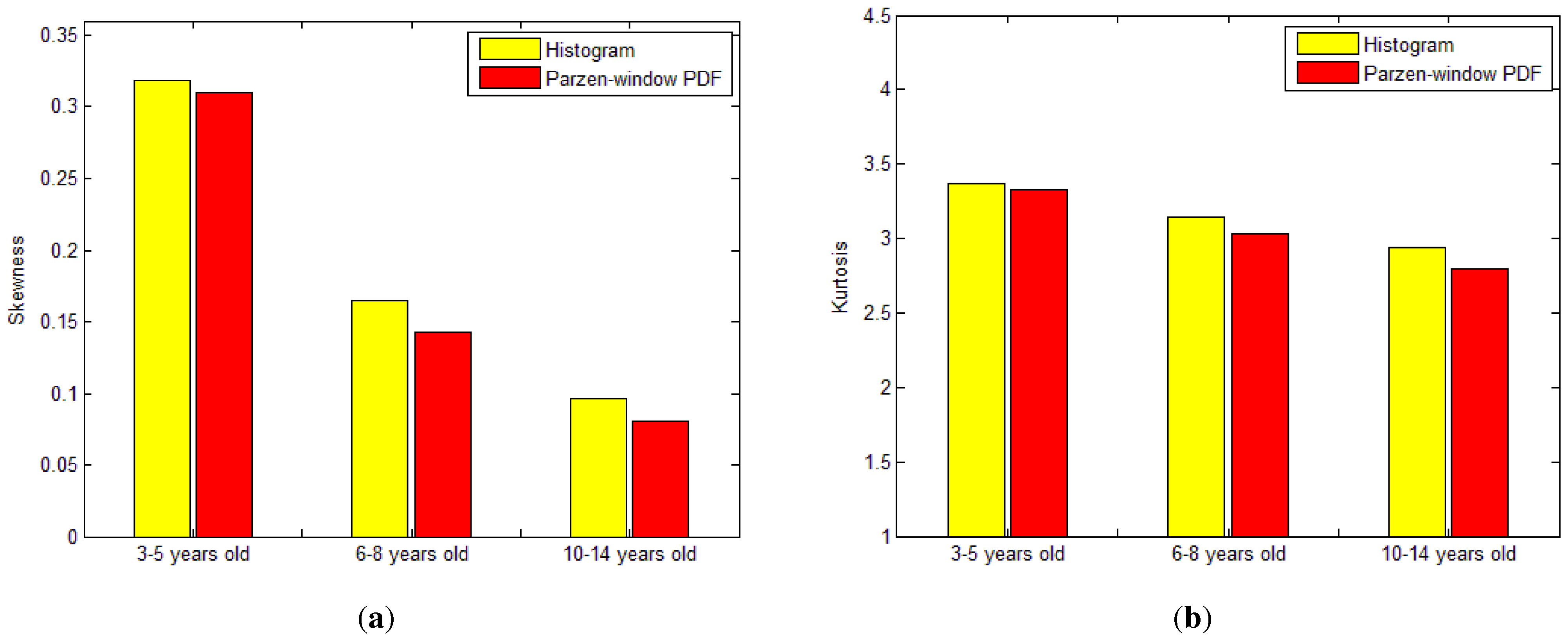
The SK and KU results of the histogram and Parzen-window PDF are provided in Figure 6 and Table 1. It can be observed that the SK values for the children aged 3–14 years are positive and age-dependent, and the SK decreases (histogram: from 0.32 to 0.1; Parzen-window PDF: from 0.31 to 0.08) when the children grow up. The right-skewed PDF indicates that the mass of the distribution is located on the left side of the figure, which implies that more than a half of the stride interval samples are lower in amplitude than the mean of the PDF (see the representative examples in Figure 1). In addition, it is worth noting from Figure 6a that the SK decreases rapidly when the children are 3–8 years old, and continues to decrease at a slower rate until the children are 14 years old. Such results confirm our inference about the development process of the locomotor control system in young children described above.
Figure 5. Illustration of four typical probability density functions (PDFs) that possess different kurtosis (KU) values: uniform distribution, dot curve, KU = 1 . 8 ; raised cosine distribution, dashed curve, KU = 2 . 41 ; Gaussian distribution, solid curve, KU = 3 ; hyperbolic secant distribution, dash-dot curve, KU = 5 . au: arbitrary units.
Entropy 15 00753 g005
Figure 6. Bar graphics of the mean values of (a) skewness (SK) and (b) kurtosis (KU) computed from the histograms and the Parzen-window probability density functions (PDFs) of the 3- to 5-year-old, 6- to 8-year-old, and 10- to 14-year-old age groups, respectively. Statistics of the skewness and the kurtosis for the three age groups are listed in Table 1.
Entropy 15 00753 g006
Table 1. Statistical parameters computed from the histograms and the Parzen-window probability density functions (PDFs) of 50 children subjects (equal number of boys and girls). Values are mean ± standard deviation (SD).
Statistical parameters3–5 years old6–8 years old10–14 years old
Skewness (SK)Histogram 0 . 32 ± 0 . 26 0 . 16 ± 0 . 28 0 . 1 ± 0 . 19
Parzen-window PDF 0 . 31 ± 0 . 25 0 . 14 ± 0 . 26 0 . 08 ± 0 . 16
Kurtosis (KU)Histogram 3 . 37 ± 0 . 72 3 . 15 ± 0 . 85 2 . 94 ± 0 . 26
Parzen-window PDF 3 . 33 ± 0 . 69 3 . 03 ± 0 . 72 2 . 79 ± 0 . 16
From Figure 6b, it can be observed that the KU values of the PDFs are higher than 3.0 (the value of Gaussian PDF in Figure 5) and lower than 5.0 (the value of hyperbolic secant PDF in Figure 5) when the children are 3–5 years old, are very close to 3.0 when the children are 6–8 years old, and are between 2.41 (the value of raised cosine PDF in Figure 5) and 3.0 when the children are 9–14 years old. Such results indicate that the PDF curves become smoother and smoother during the course of musculoskeletal growth in children, and the distributions of the stride-to-stride interval in children are not heavily concentrated on the means of the corresponding PDFs. It may be inferred that the musculoskeletal growth enables the children to better control the strides at different speeds.

4. Discussion

Statistical analysis of gait dynamics based on PDFs can provide more accurate quantitative parameters of gait that may affect the analytic inference or medical decision. The popular computing of averaged stride time and other gait parameters does not consider the underlying probability distributions of these random variables. Arithmetic calculation of the mean value by simple averaging (similar does the standard deviation) assumes the equal probability of occurrence (i.e., the uniform distribution) in data samples. However, the uniform distribution does not commonly occur in practical applications. Therefore, the mean and standard deviation computed by weighted averaging with the estimated probability of occurrence are more accurate than the simple calculation, which is widely accepted in statistics.
The PDF-based analysis methods are also useful for classification of gait patterns associated with neurodegenerative diseases [21,22]. Wu and Krishnan [21] computed the SD value from the PDF of stride interval in Parkinson’s disease and the signal turns count parameter from the stride interval time series. The least-squares support vector machine with nonlinear kernels was able to provide an accurate rate of 90.32% in the classification of gait patterns in Parkinson’s disease [21]. Wu and Shi [22] computed the modified Kullback–Leibler divergence to measure the difference between the left-foot and right-foot PDFs of stride interval, for the subject groups of healthy controls and patients with amyotrophic lateral sclerosis. They reported that the modified Kullback–Leibler divergence value is significant larger for patients with amyotrophic lateral sclerosis than for healthy controls, which implied the stride asymmetry in amyotrophic lateral sclerosis [22]. Besides the mean and SD values, the information entropy can also be computed from the estimated PDF. Rangayyan and Wu [27] used the Parzen-window method to establish the PDF models of knee joint vibroarthrographic (VAG) signals, and computed the Shannon entropy of the PDFs for the VAG signals with knee joint disorders. The related studies [27,29,30] demonstrated that the performance of classifiers can be greatly improved with the statistical parameters computed from the PDFs and the fractal dimensions of power spectral density. It is positively believed that the nonparametric PDF modeling method has high potential in the statistical analysis of biomedical signals, and the measures of gait and postural parameters for other movement disorders.
In addition to the observations of Hillman et al. [1] and Sutherland et al. [6] that the normalized temporo-spatial gait parameters are relatively mature across the age range of 7–11 years, the skewness and kurtosis parameters computed based on the Parzen-window PDFs suggested a coordination of gait dynamics still occurs until 14 years old.
The present study has some limitations that also signify the future research directions. Although the gender of the young children was matched, the number of subjects within each age group was not very large. Therefore, the results of gait analysis in the present study are still somewhat biased. On the other hand, only the stride interval time series were recorded in the experiments, hence the statistical parameters computed from one stride to another cannot provide more precise information about the dynamics in the detailed stride phases, such as stance, swing, double support, and so forth. Since the follow-up tracking experiments of gait monitoring in 50 individual children were not carried out, the present study is not able to support the long-term study on subtle changes in gait dynamics within each subject. In addition, the experiment protocol required a gait monitoring duration of 8 min for each subject, such that the very young children might pause during the continuous walking due to fatigue, which would result in the stride outliers as detected in the present study. The future study could simplify the experimental set-up for the walking monitoring of a shorter duration, the stride interval PDFs estimated from the short-range time series can then be compared with the current PDFs of long-range time series in statistical sense, to determine the appropriate duration of the gait monitoring for young children. The future work would also focus on the ranges of statistical parameters for young children in different age groups. It should require recruiting more participants in the experiments, also including the subjects with movement disorders. Quantitative study based on a large-size database could help represent the subtle changes in gait maturation, and characterize the effects of neuromuscular diseases in the locomotor control of children with movement disorders.

5. Conclusion

As Montero-Odasso et al. mentioned in the recent survey [31], gait assessment is a complementary approach for the cognition study toward better understanding of the motor function and falling risks. Gait dynamics analysis also facilitates further discrimination between the immature walking and the abnormal gait due to neurological disorders (e.g., the spastic hemiplegic cerebral palsy [32]) in children. The Parzen-window method does not require a pre-defined probability model and makes the estimated PDF closer to the distribution in nature, such that the probability density function modeling supports the measurement of temporal-spatial gait parameters with a higher degree of accuracy. The present study used the nonparametric Parzen-window method to estimate the stride interval PDF models for 50 young children in three different age groups. The results showed the changing trends of the mean and the variance of stride interval within the age range of 3–14 years. Analysis of the PDF moments (i.e., skewness and kurtosis) indicated that the musculoskeletal growth enhances the gait cadence modulation capability of young children. Notwithstanding that the statistical moments were extended for the gait dynamics analysis in the present study, there still remains a key unanswered question regarding how much the developing motor neurons and the musculoskeletal growth contribute to children’s unstable walking respectively. Future work of gait maturation could combine the studies on joint dynamics [33] of healthy young children.

Acknowledgements

This work was supported by the Fundamental Research Funds for the Central Universities of China (grant no. 2010121061), the Natural Science Foundation of Fujian (grant no. 2011J01371), and the National Natural Science Foundation of China (grant no. 81101115). N. Xiang was supported by Xiamen University Undergraduate Innovation Training Project (grant no. XDDC201210384072). Z. T. Zhong was supported by the Fundamental Research Funds for the Central Universities (grant no. CXB2011023). J. He was supported by the Xiamen University undergraduate student innovative experiment project (grant no. XDDC2011007). The authors acknowledge Hausdorff et al. for providing the data of gait experiments with public access via PhysioNet.

References

  1. Hillmana, S.J.; Stansfieldb, B.W.; Richardsonc, A.M.; Robb, J.E. Development of temporal and distance parameters of gait in normal children. Gait Posture 2009, 29, 81–85. [Google Scholar] [CrossRef] [PubMed]
  2. Sutherland, D. The development of mature gait. Gait Posture 1997, 6, 163–170. [Google Scholar] [CrossRef]
  3. Hausdorff, J.M.; Zemany, L.; Peng, C.K.; Goldberger, A.L. Maturation of gait dynamics: Stride-to-stride variability and its temporal organization in children. J. Appl. Physiol. 1999, 86, 1040–1047. [Google Scholar] [PubMed]
  4. Holt, K.G.; Saltzman, E.; Ho, C.L.; Ulrich, B.D. Scaling of dynamics in the earliest stages of walking. Phys. Ther. 2007, 87, 1458–1467. [Google Scholar] [CrossRef] [PubMed]
  5. Beck, R.J.; Andriacchi, T.P.; Kuo, K.N.; Fermier, R.W.; Galante, J.O. Changes in the gait patterns of growing children. J. Bone Joint Surg.Am. 1981, 63, 1452–1457. [Google Scholar] [PubMed]
  6. Sutherland, D.; Olshen, R.A.; Biden, E.N.; Wyatt, M.P. The Development of Mature Walking; MacKeith: Oxford, UK, 1988. [Google Scholar]
  7. Norlin, R.; Odenrich, P.; Sandlund, B. Development of gait in the normal child. J. Pediatr. Orthop. 1981, 1, 261–266. [Google Scholar] [CrossRef] [PubMed]
  8. Menkveld, S.R.; Knipstein, E.A.; Quinn, J.R. Analysis of gait patterns in school-aged children. J. Pediatr. Orthop. 1988, 8, 263–267. [Google Scholar] [CrossRef] [PubMed]
  9. Holt, K.G.; Saltzman, E.; Ho, C.L.; Kubo, M.; Ulrich, B.D. Discovery of the pendulum and spring dynamics in the early stages of walking. J. Motor Behav. 2006, 38, 206–218. [Google Scholar] [CrossRef] [PubMed]
  10. Manabe, Y.; Honda, E.; Shiro, Y.; Sakai, K.; Kohira, I.; Kashihara, K.; Shohmori, T.; Abe, K. Fractal dimension analysis of static stabilometry in Parkinson’s disease and spinocerebellar ataxia. Neurol. Res. 2001, 23, 397–404. [Google Scholar] [CrossRef] [PubMed]
  11. Doyle, T.L.; Newton, R.U.; Burnett, A.F. Reliability of traditional and fractal dimension measures of quiet stance center of pressure in young, healthy people. Arch. Phys. Med. Rehabil. 2005, 86, 2034–2040. [Google Scholar] [CrossRef] [PubMed]
  12. Cimolin, V.; Galli, M.; Rigoldi, C.; Grugni, G.; Vismara, L.; Mainardi, L.; Capodaglio, P. Fractal dimension approach in postural control of subjects with Prader-Willi syndrome. J. NeuroEng. Rehabil. 2011. [Google Scholar] [CrossRef] [PubMed]
  13. Shumway-Cook, A.; Woollacott, M.H. Motor Control: Theory and Practical Applications, 2nd ed.; Lippincott Williams & Wilkins: Philadelphia, PA, USA, 2000. [Google Scholar]
  14. Wu, Y.F.; Zhong, Z.T.; Lu, M.; He, J. Statistical analysis of gait maturation in children based on probability density functions. Proc. 33rd Annu. Int. Conf. IEEE Eng. Med. Biol. Soc. 2011, 1652–1655. [Google Scholar]
  15. Moody, G.B.; Mark, R.G.; Goldberger, A.L. PhysioNet: A web-based resource for the study of physiologic signals. IEEE Eng. Med. Biol. Mag. 2001, 20, 70–75. Available online: http://www.physionet.org/. [Google Scholar] [CrossRef] [PubMed]
  16. Hausdorff, J.M.; Ladin, Z.; Wei, J.Y. Footswitch system for measurement of the temporal parameters of gait. J. Biomechan. 1995, 28, 347–351. [Google Scholar] [CrossRef]
  17. Wu, Y.F.; Krishnan, S. Computer-aided analysis of gait rhythm fluctuations in amyotrophic lateral sclerosis. Med. Biol. Eng. Comput. 2009, 47, 1165–1171. [Google Scholar] [CrossRef] [PubMed]
  18. Hahn, G.J.; Shapiro, S.S. Statistical Models in Engineering; Wiley: Hoboken, NJ, USA, 1994. [Google Scholar]
  19. Scott, D.W. On optimal and data-based histograms. Biometrika 1979, 66, 605–610. [Google Scholar] [CrossRef]
  20. Parzen, E. On estimation of a probability density function and mode. Ann. Math. Stat. 1962, 33, 1065–1076. [Google Scholar] [CrossRef]
  21. Wu, Y.F.; Krishnan, S. Statistical analysis of gait rhythm in patients with Parkinson’s disease. IEEE Trans. Neural Syst. Rehabil. Eng. 2010, 18, 150–158. [Google Scholar] [PubMed]
  22. Wu, Y.F.; Shi, L. Analysis of altered gait rhythm in amyotrophic lateral sclerosis based on nonparametric probability density function estimation. Med. Eng. Phys. 2011, 33, 347–355. [Google Scholar] [CrossRef] [PubMed]
  23. Box, J.F. Gosset, fisher, and the t distribution. Am. Stat. 1981, 35, 61–66. [Google Scholar] [CrossRef]
  24. Rangayyan, R.M. Biomedical Signal Analysis: A Case-Study Approach; IEEE and Wiley: New York, NY, USA, 2002. [Google Scholar]
  25. Rangayyan, R.M.; Wu, Y.F. Screening of knee-joint vibroarthrographic signals using statistical parameters and radial basis functions. Med. Biol. Eng. Comput. 2008, 46, 223–232. [Google Scholar] [CrossRef] [PubMed]
  26. Marques de Sa, J.P. Applied Statistics Using SPSS, STATISTICA, and MATLAB; Springer-Verlag: Berlin, Germany, 2003. [Google Scholar]
  27. Rangayyan, R.M.; Wu, Y.F. Screening of knee-joint vibroarthrographic signals using probability density functions estimated with Parzen windows. Biomed. Signal Process. Control 2010, 5, 53–58. [Google Scholar] [CrossRef]
  28. Smyth, G.K. A note on modelling cross correlations: Hyperbolic secant regression. Biometrika 1994, 81, 396–402. [Google Scholar] [CrossRef]
  29. Wu, Y.F.; Krishnan, S. Combining least-squares support vector machines for classification of biomedical signals: A case study with knee-joint vibroarthrographic signals. J. Exp. Theor. Artif. In. 2011, 23, 63–77. [Google Scholar] [CrossRef]
  30. Rangayyan, R.M.; Oloumi, F.; Wu, Y.F.; Cai, S.X. Fractal analysis of knee-joint vibroarthrographic signals via power spectral analysis. Biomed. Signal Process. Control 2013, 8, 26–29. [Google Scholar] [CrossRef]
  31. Montero-Odasso, M.; Verghese, J.; Beauchet, O.; Hausdorff, J.M. Gait and cognition: A complementary approach to understanding brain function and the risk of falling. J. Am. Geriatr. Soc. 2012, 60, 2127–2136. [Google Scholar] [CrossRef] [PubMed] [Green Version]
  32. Goldberga, E.J.; Requejob, P.S.; Fowler, E.G. Joint moment contributions to swing knee extension acceleration during gait in children with spastic hemiplegic cerebral palsy. J. Biomechan. 2010, 43, 893–899. [Google Scholar] [CrossRef] [PubMed]
  33. Samson, W.; Desroches, G.; Cheze, L.; Dumas, R. 3D joint dynamics analysis of healthy children’s gait. J. Biomechan. 2009, 42, 2447–2453. [Google Scholar] [CrossRef] [PubMed]

