A Maximum Entropy Approach to Loss Distribution Analysis

Department of Economics and Management, University of Trento, via Inama 5, Trento 38122, Italy
Entropy 2013, 15(3), 1100-1117; https://doi.org/10.3390/e15031100
Submission received: 16 February 2013
/
Revised: 14 March 2013
/
Accepted: 18 March 2013
/
Published: 22 March 2013
Abstract
:In this paper we propose an approach to the estimation and simulation of loss distributions based on Maximum Entropy (ME), a non-parametric technique that maximizes the Shannon entropy of the data under moment constraints. Special cases of the ME density correspond to standard distributions; therefore, this methodology is very general as it nests most classical parametric approaches. Sampling the ME distribution is essential in many contexts, such as loss models constructed via compound distributions. Given the difficulties in carrying out exact simulation, we propose an innovative algorithm, obtained by means of an extension of Adaptive Importance Sampling (AIS), for the approximate simulation of the ME distribution. Several numerical experiments confirm that the AIS-based simulation technique works well, and an application to insurance data gives further insights in the usefulness of the method for modelling, estimating and simulating loss distributions.
1. Introduction
The Maximum Entropy (ME) method is a powerful non-parametric technique for density approximation, first proposed by [1] in an information theory setup. By maximizing the Shannon’s entropy contained in the data subject to moment constraints, it provides the best-fitting distribution given that the only information available are the first k empirical moments, where “best-fitting” is defined in terms of maximum entropy. An appealing feature is that, besides working well in setups where a parametric approach would fail, the ME density nests most commonly used parametric distributions. Thus, when the true data generating process is a parametric model but the investigator is unable or unwilling to assume it a priori, the ME density identifies it a posteriori, i.e., according to the empirical properties of the data. It also provides a rough measure of the distance between a specific parametric model and the true data-generating process, estimated by the ME distribution. In other words, the method gives a “data-driven” indication whether a parametric or a non-parametric approach should be employed. This is a distinctive feature that makes it more interesting than other non-parametric techniques.
Estimation of the ME distribution may be performed in a relatively straightforward manner by means of a sequential updating algorithm proposed by [2]. On the other hand, exact simulation is not trivial. In general, the distribution function does not exist in closed form, so that the inverse transform method is computationally very expensive. An accept-reject scheme can be used for specific versions of the ME density (that is, for any given value of the parameters and of the number of constraints k), but is difficult to set up in general, because the density can have very different tail behaviors, and therefore an instrumental density that works when the tail is heavy would be inefficient for light-tailed versions of the distribution. Thus, the method would require different implementations for each member of the ME family, making it quite impractical.
In this paper we resort to Adaptive Importance Sampling (AIS) for approximate simulation of the ME density. The version of AIS based on mixture distributions was first introduced by [3]. [4] extend it to general mixture classes; recently, it has been employed for estimation of cosmological parameters [5] and for simulating copulas [6]. The method is a generalization of standard Importance Sampling (IS) because, at each iteration, a sample is simulated from the instrumental density and used to improve the IS density itself. So, “adaptivity” means that the instrumental density sequentially provides a progressively better approximation of the target density. It also rigorously formalizes the well-known capacity of mixtures to approximate most distributions.
The implementation of AIS proposed by [3] is based on mixtures of normal or Student-t densities. In this paper we develop a modification using mixtures of lognormal distributions, which is necessary for the simulation of densities supported on . The AIS-based simulation methodology fits perfectly the ME setup, because it only requires the knowledge of the density function. Moreover, it is easily implemented, being based on simulation of lognormal random variables, and extremely accurate, as will be shown by means of numerical experiments.
The ME density is especially appropriate as a model for loss distributions in contexts where there are no theoretical reasons for choosing a specific parametric model. So, for example, even though the ME approach can give a satisfactory approximation of the P&L distribution of the log-returns obtained from equity prices, in this case the distribution is expected to be normal from standard financial theory, which is largely based on the hypothesis of Geometric Brownian Motion in continuous time. Thus, the use of the ME approach (similarly to the use of other ad hoc parametric distributions) is grounded on empirical reasons, but may be difficult to justify theoretically. On the other hand, the distribution of claims in non-life insurance or losses in operational risk is usually not expected to belong to any specific parametric family, and therefore, in absence of theoretical a priori information about the model, a non-parametric methodology such as ME can be very useful, as the choice has to be mostly motivated by the empirical features of the data. Finally, from the point of view of risk management, being able of sampling the ME distribution is crucial: although in simple cases risk measures can be computed by numerical integration, in a loss model obtained via compound distribution simulation is often the only way of measuring risk.
The main contribution of this paper is threefold. First, we extend the AIS methodology to the setup where the target distribution is supported on , instead of . Second, we use this technique for approximate simulation of the ME density. In this way, we overcome the difficulties encountered in exact simulation of the ME distribution. Finally, we show that the combination of ME and AIS provides an effective non-parametric approach for modelling different kinds of loss distributions and assessing the improvement with respect to classical parametric distributions.
The rest of this work is organized as follows. Section 2 reviews the ME method. Section 3 details the AIS approach to the simulation of the ME density. Section 4 shows selected results of the simulation experiments and applies the technique to the estimation and simulation of the distribution of indemnity payments. A thorough analysis of this example shall show the precision of the AIS simulation method and the merits of the ME approach in fitting the data and identifying the appropriateness or inappropriateness of standard parametric approaches. Finally, Section 5 concludes.
2. Background about the Maximum Entropy Method
The Maximum Entropy method is best described by Jaynes’ (1957) words: the ME distribution is “uniquely determined as the one which is maximally noncommittal with respect to missing information, and it agrees with what is known, but expresses maximum uncertainty with respect to all other matters”. The ME density takes the form
where k is the number of moment constraints and s are the functional forms of the so-called “characterizing moments”. In most cases, they are the arithmetic or logarithmic moments, corresponding respectively to and , but other choices are possible [7]. The parameters are customarily defined using the Greek letter λ because they are the Lagrange multipliers obtained by solving the maximization problem
under the constraints
where f is a density, W is the Shannon entropy associated to f and is the sample counterpart of the i-th characterizing moment. It can be shown [7] that the solution, called ME density, takes the form Equation (1).
Despite its interesting properties, only very recently the method has been used more extensively in economics and finance ([8,9,10,11,12,13]). One reason is that Equation (2) cannot be solved analytically for , and the preferred algorithm for finding a solution, namely the Newton–Raphson algorithm, requires a very precise initialization to reach convergence, even for moderately large k [2]. However, [2] has developed a generalization of the algorithm that makes it easier to find the optimal density. The idea is that there is no need to impose all the moment constraints simultaneously. Instead, one can impose the constraints one at a time, from the lowest to the highest moment, and update the ME density sequentially, every time a new constraint is taken into account. The advantage of such a procedure is twofold: first, the maximization subject to few moment constraints can be easily carried out with standard Newton–Raphson. Second, the moments are not independent, so that the estimates of the first k parameters will typically be little changed when considering the ME density of order , and can therefore be used as starting values for the ()-order problem.
The other relevant problem in practical applications is the choice of the “optimal” value of k. In general, a larger number of constraints results in a more precise approximation, but the estimation of more parameters introduces further noise and may lead to overfitting. There are two possible ways of proceeding.
Since the maximized log-likelihood is equal to , where the s are the parameters of the fitted ME(k) density and n is the sample size, a log-likelihood ratio (llr) test is easily computed. The test of the hypothesis () against is given by ; from standard limiting theory, its asymptotic distribution is . The model-selection procedure would thus be based on the following steps: (a) estimate sequentially the ME density with ; (b) perform the test for each value of s; (c) stop at the first value of s (, say) such that the hypothesis cannot be rejected and conclude that the optimal value of k (from now on denoted by ) is equal to .
The preceding solution does not take into account the cost of estimating a model with a larger number of parameters. A possible remedy consists in computing an information criterion, such as the Akaike (AIC) or Bayesian (BIC) Information Criterion. To avoid overfitting, one can stop at the value such that at least one of the following two conditions holds: (1) the llr test cannot reject the hypothesis ; (2) the numerical value of AIC [or BIC] is larger than the numerical value of AIC [or BIC]. In the following we will mostly employ this approach.
The ME method is practically very important when the distribution to be approximated is non-standard, with features such as high skewness and/or kurtosis and heavy tail: in this case the ME distribution is able to catch them, whereas a standard parametric model would fail. In the latter case, it may be necessary to consider many terms in the exponent of the ME density, with the consequence that application of standard Newton–Raphson is unfeasible and Wu’s (2003) sequential algorithm is the only way of estimating the parameters.
On the other hand, classical distributions, such as the normal, lognormal, exponential, Pareto and others are obtained (exactly) from Equation (1) for small values of k, so that if the empirical distribution is “similar” to one of them, usually one or two moments will suffice to find a very good approximation. In this case estimation results based on the ME distribution and on the correct parametric model are essentially the same.
For the purposes of risk analysis of loss models, the most important distributions encompassed by the ME distribution are the lognormal and the Pareto. The lognormal is a logarithmic ME density with ; the values of the parameters are
The Pareto is a logarithmic ME density with and parameters
See [7] for further details as well as for other examples.
This discussion suggests to use the ME approach as a procedure for verifying the appropriateness of a certain parametric model and/or assessing the distance of the data at hand from a given distribution: for example, when the investigator is uncertain between the Pareto and the lognormal distribution, a possible way of proceeding consists in fitting sequentially the ME(k) distribution with , stopping at the smallest value of k such that the llr test cannot reject the null hypothesis. The data-generating process is Pareto if the test accepts , lognormal if it accepts , neither Pareto nor lognormal if it accepts ; moreover, a large value of k implies a large difference between the lognormal and the fitted ME distribution. See [14] for details.
3. Approximate Simulation of the ME Distribution
The ME distribution function does not exist in closed form, because the density (1) cannot be integrated analytically. Resorting to numerical integration may be reasonable for computing quantiles of X, but is rather cumbersome for the implementation of the inverse transform method. On the other hand, the flexibility of the ME distribution and, in particular, its widely varying tail-heaviness, make it difficult to find an envelope instrumental distribution general enough to set up an accept-reject scheme that works efficiently for any ME density.
Given these difficulties in simulating the ME distribution exactly, we propose a method based on Adaptive Importance Sampling (AIS; see [15,16,17]). The implementation of AIS used here was developed by [3,4] in a Bayesian setup and can also be used for approximate simulation of any absolutely continuous random variable [6]. Instead of a fixed IS density g, AIS finds a sequence of importance densities () aimed at approximating the target density f. Thus, even starting from an initial instrumental density that is quite different from the optimal one, the algorithm eventually provides the most efficient (in a sense that shall be clarified below) IS density. A pseudo-code description of the algorithm is as follows:
- Simulate a first sample by means of standard IS; compute the IS weights ().
- Use this sample to approximate the moments of f and construct the updated importance function .
- Measure the goodness of the approximation by means of the relative entropy (or Kullback–Leibler divergence; see ([18][Section 3.3]) from the target:
- “Adjust” the density so that . More formally, compute , where θ is the vector of parameters of .
- Repeat the preceding steps until some convergence criterion is met.
The functional form of g must satisfy the requirements of being positive for all values in the support of the target and making minimization of Equation (5) as straightforward as possible. [3,4] show that a convenient instrumental density is a finite mixture of normal distributions, namely
where , and are respectively the vector of weights, expected values and variances of the D mixture components. If the target density is p-variate with , Equation (6) is a p-variate normal mixture and the dimensions of the normal parameters change accordingly.
All parameters of Equation (6) are adaptable, that is, they are supposed to be updated at each iteration of the algorithm. Furthermore, it is possible to use mixtures of different densities: [3,4] extend the algorithm to mixtures of Student-t densities. The key issue is the minimization of the relative entropy at step 4. Clearly, this depends on the choice of the instrumental density g: a detailed analysis when g is a Gaussian mixture is presented below (see the description of Algorithm 2). We can now give a more precise formulation of the algorithm.
| Algorithm 1 (Adaptive Importance Sampling) |
|
An approximate sample from the target density is obtained by sampling with replacement from and weighting the observations by means of the vector . This algorithm cannot be, however, directly applied to the simulation of the ME density based on logarithmic moments. The reason is that the support of a normal (or Student-t) mixture is the real line, whereas the support of the logarithmic ME density is . It follows that the approximation is necessarily bad because, when simulating from the mixture, there is a non-zero probability of obtaining negative values. To overcome this difficulty, we need an instrumental distribution with support , with and . Fortunately, there is a convenient solution, whose great advantage consists in leaving unchanged the updating equations obtained for a normal mixture. Assume the instrumental density is a finite mixture of lognormal distributions: , where is the lognormal density with parameters and ; it is immediate to verify that, if X has density g, the density of is Equation (6), namely a normal mixture where both the mixing weights and the parameters of the component densities are the same of g. For the setup at hand, Algorithm 1 can thus be rewritten as follows.
| Algorithm 2 (Lognormal mixture Adaptive Importance Sampling) |
|
It is worth stressing that at step 2(a) we take the logarithm of the current sample, which has a normal distribution, so that we can update π, and using the updating equations of the normal distribution. Then, at step 2(b), we use the updated values of the parameters for simulating the lognormal distribution.
The main technical issue is the update of the importance function g at each iteration. When it is a p-variate normal mixture, the algorithm works as follows. At iteration t, the importance weights associated with the sample are given by
and the normalized weights are . Let now . Similarly to [3], the update is performed by iterating, for any , the equations:
where
Convergence of the algorithm has been established by [4]. In practice, to determine a stopping criterion, the goodness of the approximation must be evaluated at each iteration. An approximate diagnostic directly related to the relative entropy Equation (5) is the normalized perplexity , where is the Shannon entropy of the normalized weights . ([4][Section 2.1]) show that is an estimator of and that . On average, the normalized perplexity increases at each iteration, so that it is reasonable to stop the algorithm when it cannot be further increased (hence the entropy cannot be further decreased). Thus, the algorithm can be stopped when the normalized perplexity does not change significantly over some (five, say) successive iterations or a predefined “large” number of iterations is reached. Alternatively, it is possible to fix in advance a perplexity value such that the algorithm stops the first time that the normalized perplexity reaches : this guarantees the desired accuracy level.
In a simulation setup such as the present one, we are interested in assessing whether the simulated data can actually be treated as generated by the ME density. To this aim, we shall also test the discrepancy between the simulated data and the cdf of the ME density, computed numerically, by means of the Kolmogorov–Smirnov test.
4. Simulation and Application
In this section we perform some simulation experiments and analyze a real dataset with four aims: (i) determining the goodness of fit of the ME distribution; (ii) studying the relationship of the goodness of fit to the number of moment constraints k; (iii) evaluating the precision of the AIS-based simulation methodology; (iv) assessing the comparative performance of the ME and of two commonly used parametric approaches.
4.1. Simulation
If the true distribution is a member of one of the parametric families encompassed by the ME density, the estimates should be equal to the values of the parameters corresponding to that family. We check this for the versions of the ME distribution corresponding to the Lognormal and Pareto distribution.
4.1.1. Simulate Lognormal
For replications, we simulate observations from the standard Lognormal distribution and fit the ME density. The Lognormal distribution is a logarithmic ME density with (see Section 2). We estimate the ME density with and use the likelihood ratio criterion to determine the appropriate value of k (, say). Using Equation (3), we know that, when and , the true values of the parameters are , and .

Table 1.
Averages of estimated parameters of the ME density across 10,000 replications of the simulation of the distribution. Sample size is at each replication.
| 1.855 | 0.926 | 0.925 | 0.905 | |
| 1 | 1.001 | 1.002 | 1.002 | |
| 0.492 | 0.493 | 0.537 | ||
| −0.000 | −0.000 | |||
| −0.008 |
Tables Table 1 and Table 2 respectively show the averages of the estimated parameters and the values of the tests; llr is the log-likelihood ratio test (p-values in parentheses) and ST is the indistinguishability test proposed by [19]. All the tests give a clear indication in favor of the ME(2) (lognormal) distribution. The values of the estimated parameters in Table 1 for also confirm that the ME coincides with the lognormal distribution.
Table 2.
Averages of the values of the tests (for llr, p-values are in parentheses) across 10,000 replications of the simulation of the distribution. Sample size is at each replication.
| llr | ST | AIC | BIC | |
|---|---|---|---|---|
| 5.058 | 5.068 | |||
| 172.590 (0) | 0.355 | 5.500 | 5.515 | |
| 0.250 (0.617) | 0.000 | 5.503 | 5.523 | |
| 0.422 (0.516) | 0.001 | 5.506 | 5.530 |
Table 3.
Averages of the values of the tests (for llr, p-values are in parentheses) across 10,000 replications of the simulation of the distribution. Sample size is at each replication.
| llr | ST | AIC | BIC | |
|---|---|---|---|---|
| 5740.623 | 5750.411 | |||
| 0.015 (0.902) | 0.000 | 5742.394 | 5757.276 | |
| 0.058 (0.810) | 0.000 | 5743.412 | 5763.355 | |
| 0.060 (0.806) | 0.000 | 5744.478 | 5769.333 |
Table 4.
Averages of estimated parameters of the ME density across 10,000 replications of the simulation of the distribution. Sample size is at each replication.
| −2.834 | −2.879 | −3.101 | −3.583 | |
| 2.505 | 2.538 | 2.764 | 3.362 | |
| −0.006 | −0.076 | −0.331 | ||
| 0.007 | 0.051 | |||
| −0.003 |
4.1.2. Simulate Pareto
For replications, we simulate observations from the Pareto distribution with scale and shape and fit the ME density. The Pareto distribution is a logarithmic ME density with (see Section 2): in particular, from Equation (4), and . We estimate the ME density with and use the likelihood ratio criterion to determine . All the tests in Table 3 strongly suggest , i.e., a Pareto distribution, and the average estimated parameter values in Table 4 obtained for are in good agreement with the theoretical values corresponding to and .
4.1.3. Simulate a Lognormal–Pareto Mixture
To assess how well the ME method fits a non-standard distribution, we simulate a mixture of a right-truncated lognormal and a Pareto distribution. The density is given by
where Φ is the cdf of the normal distribution, and are the and the densities and is the indicator function of the set A. If we impose the condition that the density be continuous and differentiable at c, the lognormal expected value μ and the mixing weight r are no longer free parameters; in particular, they are given by [20]:
In this case, estimating the parameters of the true data-generating process in a parametric approach is rather difficult, and the ME method is an appealing alternative. The model-selection strategy fits sequentially the ME density with , computes the llr test and the BIC criterion, stops at the first value of k (, say) such that either the llr test cannot reject the hypothesis or and concludes that is equal to . As before, in the simulation experiment we use replications and sample size ; moreover, we set , and , resulting in and .
Table 5.
Averages of estimated parameters of the ME density across 10,000 replications of the simulation of the Lognormal–Pareto mixture distribution. Sample size is at each replication.
| 0.654 | 8.772 | 14.398 | 18.295 | 12.552 | 4.458 | 8.703 | 14.827 | 22.264 | −71.207 | |
| 1.380 | −5.372 | −12.024 | −17.483 | −6.895 | 11.823 | −0.512 | −20.404 | −45.028 | 347.685 | |
| 1.223 | 3.682 | 6.345 | −0.968 | −17.743 | −3.542 | 22.756 | 56.542 | −641.972 | ||
| −0.286 | −0.821 | 1.553 | 9.054 | 0.580 | −18.050 | −43.331 | 652.963 | |||
| 0.037 | −0.326 | −2.101 | 0.752 | 8.533 | 19.917 | −413.034 | ||||
| 0.021 | 0.233 | −0.312 | −2.280 | −5.482 | 170.761 | |||||
| −0.010 | 0.045 | 0.342 | 0.901 | −46.851 | ||||||
| −0.002 | −0.027 | −0.085 | 8.446 | |||||||
| 0.001 | 0.004 | −0.961 | ||||||||
| -0-.000 | 0.062 | |||||||||
| −0.002 |
Table 6.
Averages of the values of the tests (for llr, p-values are in parentheses) across 10,000 replications of the simulation of the Lognormal–Pareto mixture distribution. Sample size is at each replication.
| llr | ST | AIC | BIC | |
|---|---|---|---|---|
| 85031.171 | 85046.559 | |||
| 13563.365 (<0.001) | 0.491 | 71470.822 | 71492.978 | |
| 842.316 (<0.001) | 0.041 | 70630.336 | 70658.398 | |
| 68.841 (<0.001) | 0.003 | 70563.734 | 70599.448 | |
| 28.944 (<0.001) | 0.001 | 70536.392 | 70579.887 | |
| 29.659 (<0.001) | 0.001 | 70508.056 | 70559.811 | |
| 3.692 (0.055) | <0.001 | 70506.924 | 70564.493 | |
| 2.286 (0.131) | <0.001 | 70506.664 | 70571.292 | |
| 3.049 (0.081) | <0.001 | 70505.268 | 70577.853 | |
| 896.16 (<0.001) | <0.001 | 70511.546 | 70585.093 |
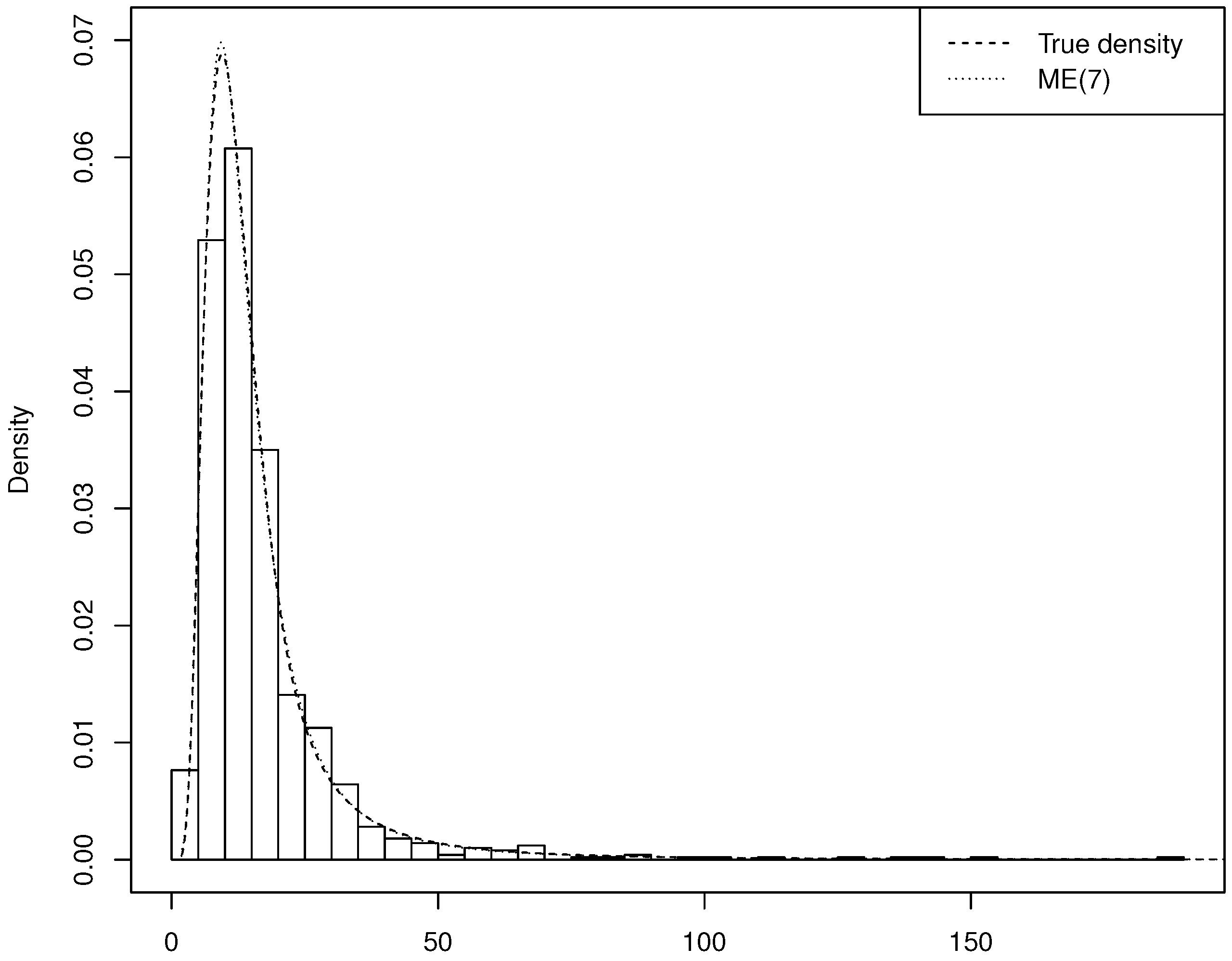
The averages of the estimated parameters and the values of the tests are reported in Table 5 and Table 6. The llr test is marginally significant for and non-significant for ; the BIC also suggests . Figure 1 displays the histogram of the simulated data superimposed with the Lognormal–Pareto mixture and the ME(7) density; for readability, in the graph we only show the observations smaller than 200. The fit is extremely good, as the two densities are virtually indistinguishable. The ME(6) density, not shown in the graph, is essentially identical to the ME(7), so that choosing would be appropriate as well.
Figure 1.
The simulated Lognormal–Pareto observations, the true Lognormal–Pareto mixture density and the fitted ME(7) density.
Figure 1.
The simulated Lognormal–Pareto observations, the true Lognormal–Pareto mixture density and the fitted ME(7) density.
4.2. Application
In Section 4.1 we have studied numerically some properties of the ME estimation methodology. Now we turn to the AIS simulation method. Thus, after finding the ME density that best fits a loss dataset, we implement AIS simulation of the estimated ME distribution and evaluate its performance; finally, we perform a risk assessment and a comparison with standard parametric models.
4.2.1. The General Liability Claims Dataset: Estimation and Simulation
For the empirical analysis, we use a loss dataset from the insurance field. The data consist of indemnity payments (losses) in USD and are available in the package evd [21]. We find it more convenient to divide the original data by 1000, so that in the following the observations are in thousands of USD. The analysis consists of four steps:
- Estimate the ME density.
- Simulate the estimated ME density;
- Compute the Kolmogorov–Smirnov (KS) distance and the significance level;
- Estimate tail probabilities using various models and compare the outcomes.
As concerns the implementation of these three steps, some remarks are in order. The fitted ME density is only non-zero for , where and are respectively the smallest and the largest observation. On the other hand, the AIS procedure based on lognormal densities simulates random numbers on . As a result, the efficiency of the algorithm is reduced, because all the simulated observations not belonging to have zero weight. Thus, it would be better to define the ME density on . Such an extension can be constructed as follows. First, estimate the parameters . The corresponding ME density is defined on , and can be seen as a truncated version of the ME density f defined on . Thus, it must exist such that . The value of can be found by solving numerically for the equation , and the density is the extension of the estimated ME density from to .
We now proceed to the estimation of the ME density. The results shown in Table 7 are not univocal: according to the llr p-value, the test for is marginally significant, is rejected and is accepted. On the other hand, the AIC and BIC criteria would both suggest . According to the model-selection criterion in Section 2, we conclude that .
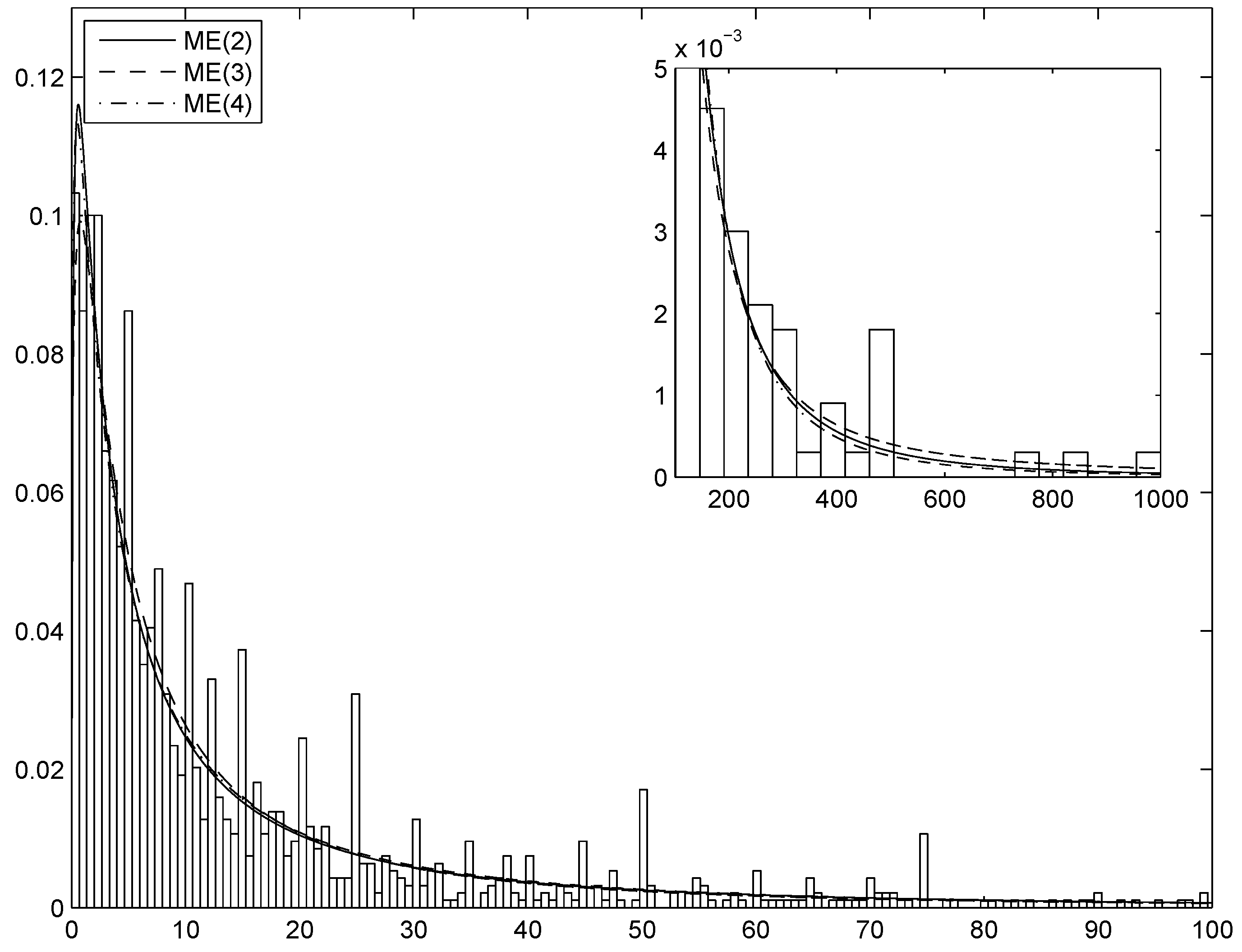
Figure 2 shows the estimated ME(2), ME(3) and ME(4) densities superimposed on the normalized histogram of the data smaller than 100. The inset focuses on the tail of the distribution, i.e., the observations larger than 100. The main differences between the distributions are concentrated in the left tail, which is not particularly important for risk analysis purposes. On the other hand, the differences in the right tail, shown in the inset, are very small (note the different scale in the main graph and in the inset): the ME(2), ME(3) and ME(4) densities are respectively equal to , and when (the largest claim in the sample).
| k | llr | p-value | AIC | BIC |
|---|---|---|---|---|
| 1 | 13345.157 | 13355.781 | ||
| 2 | 1569.080 | 11778.075 | 11794.012 | |
| 3 | 4.213 | 0.040 | 11775.878 | 11797.126 |
| 4 | 20.254 | 11757.628 | 11784.199 | |
| 5 | 0.128 | 0.721 | 11759.495 | 11791.378 |
| 6 | 0.787 | 0.374 | 11760.726 | 11797.987 |
Figure 2.
The histogram of the General Liability Claims data with the estimated ME(3), ME(4) and ME(5) densities.
Figure 2.
The histogram of the General Liability Claims data with the estimated ME(3), ME(4) and ME(5) densities.
Next we simulate the ME density using AIS. The algorithm is implemented with and with the following starting values:
With several different initializations the algorithm always converges to the same parameter values. It therefore seems that the starting values are not particularly important, a result not unexpected because the EM algorithm is quite insensitive to the initial values of the parameters [22].
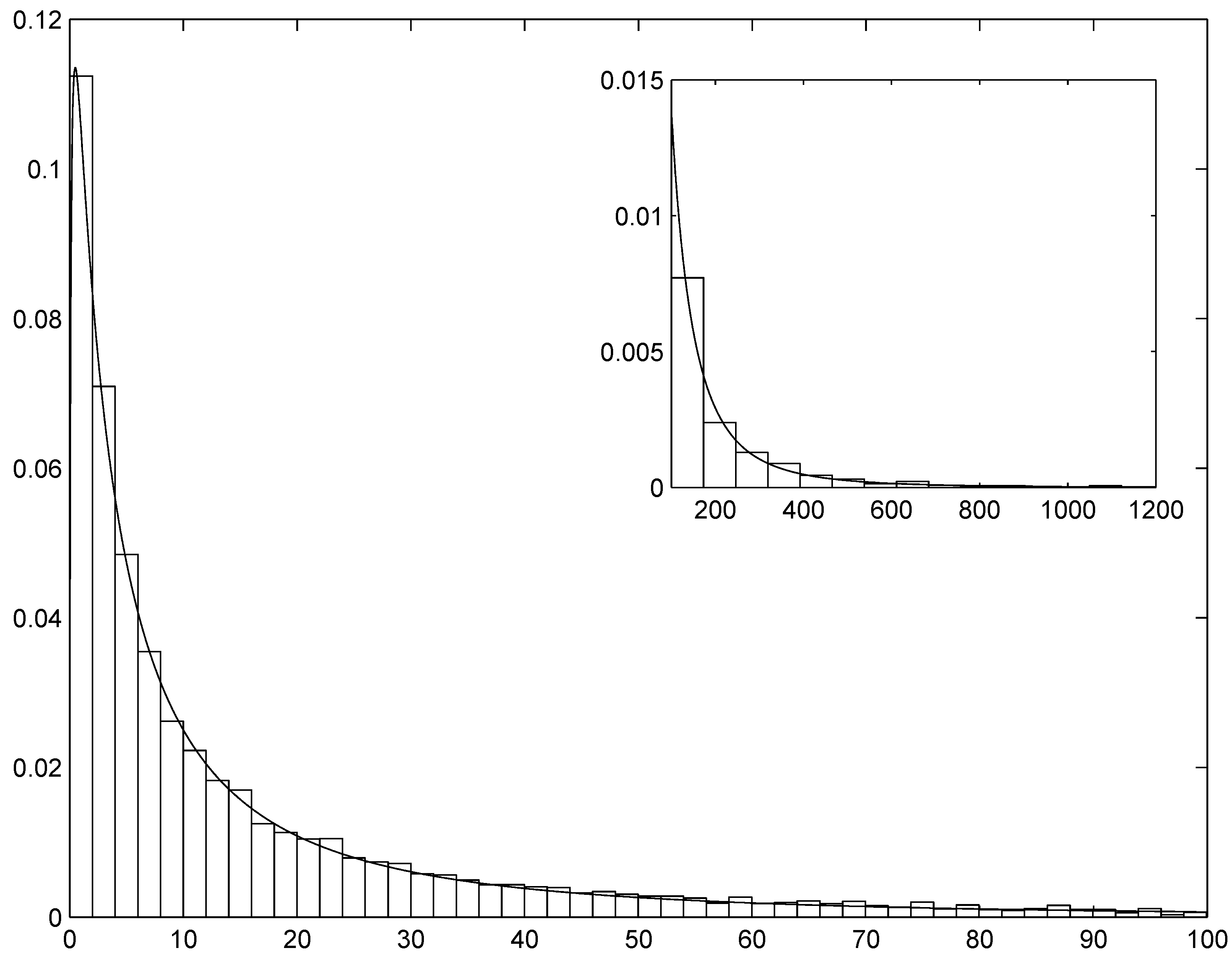
We simulate observations obtaining a normalized perplexity equal to 0.9981 at the 17-th iteration, a large value that guarantees a very high precision level. Figure 3 displays the estimated ME(4) density superimposed on the normalized histogram of the simulated observations. The graph confirms that the fit is excellent. As a final check, we compute the one-sample Kolmogorov–Smirnov test , where is the empirical cdf of the simulated data and is the theoretical cdf of the estimated ME(4) distribution. We got , whose p-value is 0.289. Thus, we accept the hypothesis that the data-generating process of the simulated observations is the estimated ME(4) density.
Figure 3.
The estimated ME(4) density superimposed on the normalized histogram of the simulated observations.
Figure 3.
The estimated ME(4) density superimposed on the normalized histogram of the simulated observations.

Turning now to risk analysis, we estimate tail probabilities using the ME density and compare them with those obtained by means of traditional parametric approaches. With loss data, typical choices are the Lognormal or the Pareto distribution, depending on tail heaviness.
Specifically, for various values x between 60 and 900 we compute tail probabilities for the lognormal (which coincides with ME(2)), Pareto, ME(3) and ME(4) distributions, with the aim of assessing the robustness of the results with respect to the ME densities that we were uncertain about in the analysis carried out above. We also show the frequencies , where () are the observed losses. According to the discussion in Section 2, the Pareto distribution should be ruled out, as the llr test rejects the hypothesis at any significance level. Nonetheless, we include it either because it is a commonly used model for this kind of data or because by so doing we can check ex post whether the decision made on the basis of the ME test is correct. As often happens, the choice of the Pareto threshold u is not easy: from the mean excess function and the Hill plot we find that seems to be a reasonable compromise between bias and variance. The outcomes are shown in Table 8.
Among the distributions considered in the experiment, the ME(4) and the lognormal (i.e., ME(2)) show the minimum distances from the observed frequencies. Such a similarity is not surprising because the ME(4) is the best distribution according to the llr test and the information criteria, but the lognormal (ME(2)) is nearly accepted by the llr test. The Pareto tail is definitely too heavy, as expected from the results of the ME test. The ME(3) is heavier-tailed than the ME(4) distribution, but the difference is not dramatic.
Table 8.
Tail probabilities obtained via various ME densities and standard parametric approaches for the General Liability Claims dataset.
| Threshold | Logn(2.04, 2.54) | Par(14, 0.94) | ME(3) | ME(4) | Obs |
|---|---|---|---|---|---|
| 60 | 0.0986 | 0.2066 | 0.0990 | 0.0965 | 0.0960 |
| 80 | 0.0708 | 0.1647 | 0.0736 | 0.0676 | 0.0673 |
| 100 | 0.0537 | 0.1372 | 0.0582 | 0.0501 | 0.0493 |
| 120 | 0.0423 | 0.1177 | 0.0480 | 0.0386 | 0.0427 |
| 140 | 0.0343 | 0.1032 | 0.0408 | 0.0306 | 0.0353 |
| 160 | 0.0284 | 0.0919 | 0.0354 | 0.0249 | 0.0293 |
| 180 | 0.0239 | 0.0829 | 0.0313 | 0.0205 | 0.0267 |
| 200 | 0.0204 | 0.0756 | 0.0281 | 0.0172 | 0.0220 |
| 220 | 0.0176 | 0.0694 | 0.0255 | 0.0146 | 0.0193 |
| 240 | 0.0154 | 0.0642 | 0.0233 | 0.0125 | 0.0180 |
| 260 | 0.0135 | 0.0598 | 0.0215 | 0.0109 | 0.0160 |
| 280 | 0.0120 | 0.0559 | 0.0200 | 0.0095 | 0.0140 |
| 300 | 0.0107 | 0.0526 | 0.0187 | 0.0083 | 0.0107 |
| 350 | 0.0083 | 0.0457 | 0.0161 | 0.0062 | 0.0093 |
| 400 | 0.0066 | 0.0404 | 0.0142 | 0.0047 | 0.0073 |
| 450 | 0.0053 | 0.0363 | 0.0127 | 0.0037 | 0.0060 |
| 500 | 0.0044 | 0.0329 | 0.0116 | 0.0030 | 0.0020 |
| 550 | 0.0037 | 0.0302 | 0.0106 | 0.0024 | 0.0020 |
| 600 | 0.0031 | 0.0278 | 0.0098 | 0.0020 | 0.0020 |
| 650 | 0.0027 | 0.0259 | 0.0092 | 0.0017 | 0.0020 |
| 700 | 0.0023 | 0.0241 | 0.0086 | 0.0014 | 0.0020 |
| 750 | 0.0020 | 0.0226 | 0.0081 | 0.0012 | 0.0013 |
| 800 | 0.0018 | 0.0213 | 0.0076 | 0.0010 | 0.0013 |
| 850 | 0.0016 | 0.0201 | 0.0072 | 0.0009 | 0.0013 |
| 900 | 0.0014 | 0.0191 | 0.0069 | 0.0008 | 0.0007 |
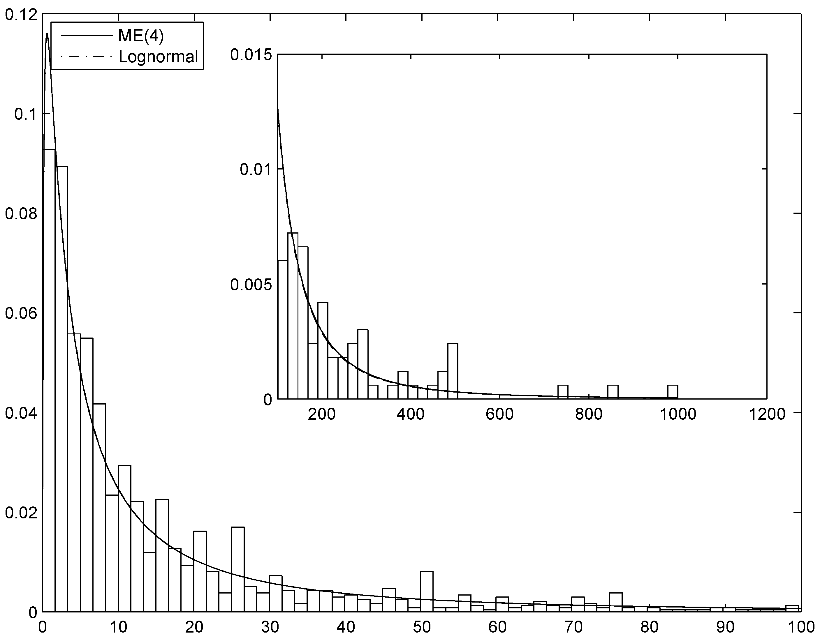
Finally, Figure 4 shows the ME(4) and the lognormal densities superimposed on the histogram of the data. The fit is very good, and the two densities are almost indistinguishable.
5. Conclusions
In this paper we have developed a non-parametric approach to loss distribution analysis based on the concept of Maximum Entropy. The main technical contribution is a flexible procedure for approximate simulation of the ME distribution, based on an extension of the Adaptive Importance Sampling algorithm introduced by [3,4]. More generally, the paper details the merits of the ME approach in the typical risk analysis process of loss distributions, from model building to estimation, simulation and risk measurement.
Figure 4.
The estimated ME(4) and lognormal densities superimposed on the histogram of the General Liability Claims observations.
Figure 4.
The estimated ME(4) and lognormal densities superimposed on the histogram of the General Liability Claims observations.
The method is appealing for various reasons. First, it allows to fit the best distribution (“best” being defined according to the Maximum Entropy principle) for the data at hand, which is particularly useful when there are no theoretical reasons for adopting a parametric distribution. Second, it may serve as a test of the choice between two (or more) parametric models. Finally, both estimation and simulation are computationally feasible.
The simulation method proposed in this paper has proved to be very precise and may be of crucial importance in models such as the compound Poisson distribution commonly used for modelling non-life insurance claims and operational losses.
A relevant topic that requires further research is the extension of the AIS instrumental density to mixtures that can approximate target distributions with support for some , such as the Pareto or the truncated lognormal distribution.
Acknowledgements
The author would like to thank Massimo Riccaboni and Stefano Schiavo for useful discussions about the ME methodology and two anonymous referees whose valuable comments greatly helped to improve the contents of this paper.
References
- Jaynes, E.T. Information theory and statistical mechanics. Phys. Rev. 1957, 106, 620–630. [Google Scholar]
- Wu, X. Calculation of maximum entropy densities with application to income distribution. J. Econom. 2003, 115, 347–354. [Google Scholar] [CrossRef]
- Cappé, O.; Guillin, A.; Marin, J.; Robert, C. Population Monte Carlo. J. Comput. Graph. Stat. 2004, 13, 907–929. [Google Scholar] [CrossRef]
- Cappé, O.; Douc, R.; Guillin, A.; Robert, C. Adaptive importance sampling in general mixture classes. Stat. Comput. 2008, 18, 447–459. [Google Scholar] [CrossRef] [Green Version]
- Wraith, D.; Kilbinger, M.; Benabed, K.; Cappé, O.; Cardoso, J.F.; Fort, G.; Prunet, S.; Robert, C. Estimation of cosmological parameters using adaptive importance sampling. Phys. Rev. D 2009, 80, 023502. [Google Scholar] [CrossRef]
- Bee, M. Adaptive importance sampling for simulating copula-based distributions. Insur. Math. Econ. 2011, 48, 237–245. [Google Scholar] [CrossRef]
- Kapur, J. Maximum Entropy Models in Science and Engineering; Wiley: New York, USA, 1989. [Google Scholar]
- Buchen, P.; Kelly, M. The maximum entropy distribution of an asset inferred from option prices. J. Financ. Quant. Anal. 1996, 31, 143–159. [Google Scholar] [CrossRef]
- Hawkins, R. Maximum entropy and derivative securities. Adv. Econ. 1997, 12, 277–301. [Google Scholar]
- Stutzer, M. A simple nonparametric approach to derivative security valuation. J. Financ. 1996, 51, 1633–1652. [Google Scholar] [CrossRef]
- Breuer, T.; Csiszár, I. Systematic stress tests with entropic plausibility constraints. J. Bank. Financ. 2013, in press. [Google Scholar] [CrossRef]
- Neri, C.; Schneider, L. Maximum entropy distributions inferred from option portfolios on an asset. Financ. Stoch. 2012, 16, 293–318. [Google Scholar] [CrossRef]
- Rodriguez, J.O.; Santosa, F. Estimation of asset distributions from option prices: Analysis and regularization. SIAM J. Financ. Math. 2012, 3, 374–401. [Google Scholar] [CrossRef]
- Bee, M.; Riccaboni, M.; Schiavo, S. Pareto versus lognormal: A maximum entropy test. Phys. Rev. E 2011, 84, 026104. [Google Scholar] [CrossRef]
- Zhang, P. Nonparametric importance sampling. J. Am. Stat. Assoc. 1996, 91, 1245–1253. [Google Scholar] [CrossRef]
- Rubinstein, R. The Cross-Entropy method for combinatorial and continuous optimization. Methodol. Comput. Appl. Probab. 1999, 2, 127–190. [Google Scholar] [CrossRef]
- Morio, J. Extreme quantile estimation with nonparametric adaptive importance sampling. Simul. Modell. Pract. Theory 2012, 27, 76–89. [Google Scholar] [CrossRef]
- Rubinstein, R.; Kroese, D. The Cross-Entropy Method; Springer: Berlin/Heidelberg, Germany, 2004. [Google Scholar]
- Soofi, E.; Ebrahimi, N.; Habibullah, M. Information Distinguishability with Application to Analysis of Failure Data. J. Am. Stat. Assoc. 1995, 90, 657–668. [Google Scholar] [CrossRef]
- Scollnik, D. On composite lognormal-Pareto models. Scand. Actuar. J. 2007, 1, 20–33. [Google Scholar] [CrossRef]
- Stephenson, A.G. evd: Extreme Value Distributions. R News 2002, 2, 31–32. [Google Scholar]
- McLachlan, G.; Krishnan, T. The EM Algorithm and Extensions, 2nd ed.; Wiley: New York, USA, 2008. [Google Scholar]
© 2013 by the author; licensee MDPI, Basel, Switzerland. This article is an open access article distributed under the terms and conditions of the Creative Commons Attribution license (http://creativecommons.org/licenses/by/3.0/).
Share and Cite
MDPI and ACS Style
Bee, M. A Maximum Entropy Approach to Loss Distribution Analysis. Entropy 2013, 15, 1100-1117. https://doi.org/10.3390/e15031100
AMA Style
Bee M. A Maximum Entropy Approach to Loss Distribution Analysis. Entropy. 2013; 15(3):1100-1117. https://doi.org/10.3390/e15031100
Chicago/Turabian StyleBee, Marco. 2013. "A Maximum Entropy Approach to Loss Distribution Analysis" Entropy 15, no. 3: 1100-1117. https://doi.org/10.3390/e15031100