On a Generalized Entropy Measure Leading to the Pathway Model with a Preliminary Application to Solar Neutrino Data

Abstract

An entropy for the scalar variable case, parallel to Havrda-Charvat entropy, was introduced by the first author, and the properties and its connection to Tsallis non-extensive statistical mechanics and the Mathai pathway model were examined by the authors in previous papers. In the current paper, we extend the entropy to cover the scalar case, multivariable case, and matrix variate case. Then, this measure is optimized under different types of restrictions, and a number of models in the multivariable case and matrix variable case are obtained. Connections of these models to problems in statistical and physical sciences are pointed out. An application of the simplest case of the pathway model to the interpretation of solar neutrino data by applying standard deviation analysis and diffusion entropy analysis is provided.

1. Introduction

Classical Shannon entropy has been generalized in many directions [1,2]. An α-generalized entropy, parallel to Havrda-Charvat entropy, introduced by the first author, is found to be quite useful in deriving pathway models [3], including Tsallis statistics [4] and superstatistics [5,6]. It is also connected to Kerride’s measure of inaccuracy [7]. For the continuous case, let $f(X)$ be a density function associated with a random variable X, where X could be a real or complex scalar, vector or matrix variable. In the present paper we consider only the real cases for convenience. Let

$$M_{\alpha }(f)=\frac{{\int }_X{[f(X)]}^{2-\alpha }\mathrm{d}X-1}{\alpha -1},\alpha \ne 1$$

(1.1)

Note that when $\alpha \to 1,M_{\alpha }(f)\to S(f)=-{\int }_{X}f(X)lnf(X)\mathrm{d}X$ where $S(f)$ is Shannon’s entropy [7] and in this sense (1.1) is a α-generalized entropy measure. The corresponding discrete case is available as

$$\frac{{\sum }_{i=1}^k{p}_i^{2-\alpha }-1}{\alpha -1},p_i>0,i=1,...,k,p_1+...p_k=1,\alpha \ne 1$$

Characterization properties and applications of (1.1) may be seen from [7]. Note that

$${\int }_X{[f(X)]}^{2-\alpha }\mathrm{d}X={\int }_X{[f(X)]}^{1-\alpha }f(X)\mathrm{d}X=E{[f(X)]}^{1-\alpha }$$

Thus there is a parallelism with Kerridge’s measure of inaccuracy. The α-generalized Kerridge’s measure of inaccuracy [9] is given by

$$\frac{{\int }_{x}P(x){[Q(x)]}^{1-\alpha }-1}{\alpha -1}=\frac{E{[Q(x)]}^{1-\alpha }-1}{\alpha -1},\alpha \ne 1$$

(1.2)

When $\alpha \to 1$, Equation (1.2) goes to Kerridge’s measure of inaccuracy given by

$$K(P,Q)=-{\int }_{x}P(x)lnQ(x)\mathrm{d}x$$

(1.3)

where x is a scalar variable, $P(x)$ is the true density and $Q(x)$ is a hypothesized or assigned density for the true density $P(x)$. Then a measure of inaccuracy in taking $Q(x)$ for the true density $P(x)$ is given by Equation (1.3) and its α-generalized form is given by Equation (1.2).

Earlier works on Shannon’s measure of entropy, measure of directed divergence, measure of inaccuracy and related items and applications in natural sciences may be seen in [7] and the references therein. A measure of entropy, parallel to the one of Havrda-Charvat entropy was introduced by Tsallis in 1988 [4,8,9], given by

$$T_{\alpha }(f)=\frac{{\int }_x{[f(x)]}^{\alpha }\mathrm{d}x-1}{1-\alpha },\alpha \ne 1$$

(1.4)

Tsallis statistics or non-extensive statistical mechanics is derived by optimizing (1.4) by putting restrictions in an escort density associated with $f(x)$ of Equation (1.4). Let $g(x)=\frac{{[f(x)]}^{\alpha }}{m},m={\int }_x{[f(x)]}^{\alpha }\mathrm{d}x<\infty$. If $T_{\alpha }(f)$ is optimized over all non-negative functional f, subject to the conditions that $f(x)$ is a density and the expected value in the escort density is a given quantity, that is ${\int }_{x}xg(x)\mathrm{d}x=$ a given quantity, then the Euler equation to be considered, if we optimize by using calculus of variations, is that

$$\frac{\partial }{\partial f}[{\left\{f(x)\right\}}^{\alpha }-{\lambda }_{1}f(x)+{\lambda }_{2}x{\left\{f(x)\right\}}^{\alpha }]=0$$

where ${\lambda }_1$ and ${\lambda }_2$ are Lagrangian multipliers. That is,

$$\alpha {[f(x)]}^{\alpha -1}-{\lambda }_1+{\lambda }_{2}x\alpha {[f(x)]}^{\alpha -1}=0$$

Then

$$f(x)=c{[1+{\lambda }_{2}x]}^{-\frac{1}{\alpha -1}},c={(\frac{{\lambda }_1}{\alpha })}^{\frac{1}{\alpha -1}}$$

Taking ${\lambda }_2=a(\alpha -1)$ for $\alpha >1,a>0$ we have Tsallis statistics as

$$f(x)=c{[1+a(\alpha -1)x]}^{-\frac{1}{\alpha -1}},\alpha >1,a>0$$

(1.5)

For $\alpha <1$, writing $\alpha -1=-(1-\alpha )$ the density in Equation (1.5) changes to

$$f_x(x)=c_1{[1-a(1-\alpha )x]}^{\frac{1}{1-\alpha }},\alpha <1,a>0$$

where $1-a(1-\alpha )x>0$ and $c_1$ can act as a normalizing constant if $f_1(x)$ is to be taken as a statistical density. Tsallis statistics in Equation (1.5) led to the development of none-extensive statistical mechanics. We will show later that Equation (1.5) comes directly from the entropy of Equation (1.1) without going through any escort density. Let us optimize Equation (1.1) subject to the conditions that $f(x)$ is a density, ${\int }_{x}f(x)\mathrm{d}x=1$, and that the expected value of x in $f(x)$ is a given quantity, that is, ${\int }_{x}xf(x)\mathrm{d}x=$ a given quantity. Then, if we use calculus of variations, the Euler equation is of the form

$$\frac{\partial }{\partial f}[{\left\{f(x)\right\}}^{2-\alpha }-{\lambda }_{1}f(x)+{\lambda }_{2}xf(x)]=0$$

where ${\lambda }_1$ and ${\lambda }_2$ are Lagrangian multipliers. Then we have

$$f_1(x)=c_1{[1-a(1-\alpha )x]}^{\frac{1}{1-\alpha }},\alpha <1,a>0$$

(1.6)

by taking $\frac{{\lambda }_2}{{\lambda }_1}=a(1-\alpha ),a>0,\alpha <1,$ and $c_1$ is the corresponding normalizing constant to make $f_1(x)$ a statistical density. Now, for $\alpha >1$, write $1-\alpha =-(\alpha -1)$, then directly from Equation (1.6), without going through any escort density, we have

$$f_2(x)=c_2{[1+a(\alpha -1)x]}^{-\frac{1}{\alpha -1}},\alpha >1,a>0$$

(1.7)

which is Tsallis statistics for $\alpha >1$. Thus, both the cases $\alpha <1$ and $\alpha >1$ follow directly from Equation (1.1).

Now, let us look into optimizing (1.1) over all non-negative integrable functionals, $f(x)\ge 0$ for all x, ${\int }_{x}f(x)\mathrm{d}x<\infty$, such that two moment-type relations are imposed on f, of the form

$${\int }_x{x}^{\gamma (1-\alpha )}f(x)\mathrm{d}x=\mathrm{given}, \mathrm{and}{\int }_x{x}^{\gamma (1-\alpha )+\delta }f(x)\mathrm{d}x=\mathrm{given}$$

(1.8)

Then the Euler equation becomes

$$\frac{\partial }{\partial f}[{\left\{f(x)\right\}}^{2-\alpha }-{\lambda }_1{x}^{\gamma (1-\alpha )}f(x)+{\lambda }_2{x}^{\gamma (1-\alpha )+\delta }f(x)]=0$$

which leads to

$$f_1^{*}(x)=c_1^{*}{x}^{\gamma }{[1-a(1-\alpha )x^{\delta }]}^{\frac{1}{1-\alpha }},a>0,\alpha <1,\delta >0,\gamma >0$$

(1.9)

for $1-a(1-\alpha )x^{\delta }>0$, by taking $\frac{{\lambda }_2}{{\lambda }_1}=a(1-\alpha ),a>0,\alpha <1$, where $c_1^{*}$ can act as the normalizing constant. Equation (1.9) is a special case of the pathway model of [3] for the real scalar positive random variable $x>0$. For $\gamma =0,\delta =1$ in Equation (1.9) we obtain Tsallis statistics of Equation (1.6) for the case $\alpha <1$. When $\alpha >1$ write $1-\alpha =-(\alpha -1)$ for $\alpha >1$ then Equation (1.9) becomes

$$f_2^{*}(x)=c_2^{*}{x}^{\gamma }{[1+a(\alpha -1)x^{\delta }]}^{-\frac{1}{\alpha -1}},\alpha >1,a>0,x>0,\delta >0$$

(1.10)

When $\alpha \to 1$ both $f_1^{*}(x)$ of Equation (1.9) and $f_2^{*}(x)$ of Equation (1.10) go to

$$f_3^{*}(x)=c_3^{*}{x}^{\gamma }{\mathrm{e}}^{-a{x}^{\delta }},a>0,\delta >0,x>0$$

(1.11)

Equation (1.10) for $\alpha >1,x>0$ is superstatistics [5,6].

2. A Generalized Measure of Entropy

Let X be a scalar, a $p\times 1$ vector of scalar random variables or a $p\times n,p\ge n$ matrix of rank n of scalar random variables and let $f(X)$ be a real-valued scalar function such that $f(X)\ge 0$ for all X and ${\int }_{X}f(X)\mathrm{d}X=1$ where $\mathrm{d}X$ stands for the wedge product of the differentials in X. For example, if X is $m\times n$, $X=(x_{ij})$ then

$$\mathrm{d}X=\prod _{i=1}^m\prod _{j=1}^n\wedge \mathrm{d}{x}_{ij}$$

where ∧ stands for the wedge product of differentials, $\mathrm{d}x\wedge \mathrm{d}y=-\mathrm{d}y\wedge \mathrm{d}x\Rightarrow \mathrm{d}x\wedge \mathrm{d}x=0$. Then $f(X)$ is a density of X. When X is $p\times n,p\ge n$ we have a rectangular matrix variate density. For convenience we have taken X of full rank $n\le p$. When $n=1$ we have a multivariate density and when $n=1,p=1$ we have a univariate density. Consider the generalized entropy of Equation (1.1) for this matrix variate density, denoted by $f(X)$, then

$$M_{\alpha }(f)=\frac{{\int }_X{[f(X)]}^{2-\alpha }\mathrm{d}X-1}{\alpha -1},\alpha \ne 1$$

(2.1)

Let $n=1$. Let us consider the situation of the ellipsoid of concentration being a preassigned quantity. Let X be $p\times 1$ vector random variable. Let $V=E[(X-E(X)){(X-E(X))}^{\prime }]>O$ (positive definite) where E denotes expected value. For convenience let us denote $E(X)=\mu$. Then $\rho =E[{(X-\mu )}^{\prime }{V}^{-1}(X-\mu )]$ is the ellipsoid of concentration. Let us optimize (2.1) subject to the constraint that $f(X)\ge 0$ is a density and that the ellipsoid of concentration over all functional f is a constant, that is, ${\int }_{X}f(X)\mathrm{d}X=1$ and ${\int }_X{[{(X-\mu )}^{\prime }{V}^{-1}(X-\mu )]}^{\delta }f(X)\mathrm{d}X=$ given, where $\delta >0$ is a fixed parameter. If we are using calculus of variation then the Euler equation is given by

$$\frac{\partial }{\partial f}[{\left\{f(X)\right\}}^{2-\alpha }-{\lambda }_{1}f(X)+{\lambda }_2{[{(X-\mu )}^{\prime }{V}^{-1}(X-\mu )]}^{\delta }f(X)]=0$$

where ${\lambda }_1$ and ${\lambda }_2$ are Lagrangian multipliers. Solving the above equation we have

$$f_1(X)=C_1{[1-a(1-\alpha ){\left\{{(X-\mu )}^{\prime }{V}^{-1}(X-\mu )\right\}}^{\delta }]}^{\frac{1}{1-\alpha }}$$

(2.2)

for $\alpha <1,a>0$ where we have taken $\frac{{\lambda }_2}{{\lambda }_1}=a(1-\alpha ),a>0,\alpha <1$ and ${(\frac{{\lambda }_1}{2-\alpha })}^{\frac{1}{1-\alpha }}=C_1$. This $C_1$ can act as the normalizing constant to make $f(X)$ in Equation (2.2) a statistical density. Note that for $\alpha >1$, we have from Equation (2.2)

$$f_2(X)=C_2{[1+a(\alpha -1){\left\{{(X-\mu )}^{\prime }{V}^{-1}(X-\mu )\right\}}^{\delta }]}^{-\frac{1}{\alpha -1}},\alpha >1,a>0$$

(2.3)

and when $\alpha \to 1$, $f_1$ and $f_2$ go to

$$f_3(X)=C_3{\mathrm{e}}^{-a{[{(X-\mu )}^{\prime }{V}^{-1}(X-\mu )]}^{\delta }}$$

(2.4)

Equation (2.4) for $\delta =1$ is the multivariate Gaussian density. If $Y=V^{-\frac{1}{2}}(X-\mu )$, where $V^{-\frac{1}{2}}$ is the positive definite square root of the positive definite matrix $V^{-1}$, then $\mathrm{d}Y={\left|V\right|}^{-\frac{1}{2}}\mathrm{d}X$ and the density of Y, denoted by $g(Y)$, is given by

$$g(Y)=C_4{\mathrm{e}}^{-a{(y_1^2+...+y_p^2)}^{\delta }},-\infty <y_j<\infty ,j=1,...,p,Y^{\prime }=(y_1,...,y_p)$$

(2.5)

and $C_4$ is the normalizing constant. This normalizing constant can be evaluated in two different ways. One method is to use polar coordinate transformation, see Theorem 1.25 of [10]. Let

$$\begin{array}{cc}\hfill y_1& =r\sin {\theta }_1\sin {\theta }_2...\sin {\theta }_{p-1}\hfill \\ \hfill y_2& =r\sin {\theta }_1...\sin {\theta }_{p-2}cos{\theta }_{p-1}\hfill \\ \hfill ⋮& =⋮\hfill \\ \hfill y_{p-1}& =r\sin {\theta }_{1}cos{\theta }_1\hfill \\ \hfill y_p& =rcos{\theta }_1\hfill \end{array}$$

where $r>0,0<{\theta }_j\le \pi ,j=1,...,p-2,0<{\theta }_{p-1}\le 2\pi$ and the Jacobian is given by

$$\mathrm{d}{y}_1\wedge ...\wedge \mathrm{d}{y}_p=r^{p-1}\{\prod _{j=1}^{p-1}|\sin {\theta }_j{|}^{p-j-1}\}\mathrm{d}r\wedge \mathrm{d}{\theta }_1\wedge ...\wedge \mathrm{d}{\theta }_{p-1}$$

(2.6)

Under this transformation the exponent ${(y_1^2+...+y_p^2)}^{\delta }={(r^2)}^{\delta }$. Hence we integrate out the sine functions. The integral over ${\theta }_{p-1}$ goes from 0 to $2\pi$ and gives the value $2\pi$, and others from 0 to π. These, in general, can be evaluated by using type-1 beta integrals by putting $\sin \theta =u$ and $u^2=v$. That is,

$$\begin{array}{cc}\hfill {\int }_0^{\pi }\sin \theta \mathrm{d}\theta & =2{\int }_0^{\pi /2}\sin \theta \mathrm{d}\theta =2{\int }_0^{1}u{(1-u^2)}^{-\frac{1}{2}}\mathrm{d}u\hfill \\ & ={\int }_0^1{v}^{1-1}{(1-v)}^{-\frac{1}{2}}\mathrm{d}v=\frac{\Gamma (1)\Gamma (1/2)}{\Gamma (3/2)}\hfill \\ \hfill {\int }_0^{\pi }{(\sin \theta )}^2\mathrm{d}\theta & =\frac{\Gamma (3/2)\Gamma (1/2)}{\Gamma (4/2)}\hfill \\ \hfill ⋮& =⋮\hfill \\ \hfill {\int }_0^{\pi }{(\sin \theta )}^{p-2}\mathrm{d}\theta & =\frac{\Gamma (\frac{p-1}{2})\Gamma (1/2)}{\Gamma (\frac{p}{2})}\hfill \end{array}$$

Taking the product we have

$$2\pi \frac{{(\sqrt{\pi })}^{p-2}}{\Gamma (\frac{p}{2})}=\frac{2{\pi }^{p/2}}{\Gamma (p/2)}$$

Hence the total integral is equal to

$$1=C_4{\left|V\right|}^{\frac{1}{2}}\frac{2{\pi }^{p/2}}{\Gamma (p/2)}{\int }_0^{\infty }{r}^{p-1}{\mathrm{e}}^{-a{r}^{2\delta }}\mathrm{d}r,\delta >0$$

Put $x=a{r}^{2\delta }$ and integrate out by using a gamma integral to get

$$C_4=\frac{\delta \Gamma (\frac{p}{2})a^{\frac{p}{2\delta }}}{{\left|V\right|}^{\frac{1}{2}}{\pi }^{p/2}\Gamma (\frac{p}{2\sigma })}$$

That is, the density is given by

$$f_3(X)=\frac{\delta a^{\frac{p}{2\delta }}\Gamma (p/2)}{{\left|V\right|}^{1/2}{\pi }^{p/2}\Gamma (\frac{p}{2\delta })}{\mathrm{e}}^{-a{[{(X-\mu )}^{\prime }{V}^{-1}(X-\mu )]}^{\delta }},\delta >0,a>0,V>O$$

(2.7)

From the above steps the following items are available: The density of $Y=V^{-\frac{1}{2}}(X-\mu )$ is available as

$$g(Y)=\frac{\delta a^{\frac{p}{2\delta }}\Gamma (\frac{p}{2})}{{\pi }^{p/2}\Gamma (\frac{p}{2\delta })}{\mathrm{e}}^{-a{(Y^{\prime }Y)}^{\delta }}$$

(2.8)

The density of $u=Y^{\prime }Y=y_1^2+...+y_p^2$, denoted by $g_1(u)$, is given by

$$g_1(u)=\frac{\delta a^{\frac{p}{2\delta }}}{\Gamma (\frac{p}{2\delta })}{u}^{\frac{p}{2}-1}{\mathrm{e}}^{-a{u}^{\delta }},\delta >0,u>0$$

(2.9)

and the density of $r>0$, where $r^2=u=Y^{\prime }Y$, denoted by $g_2(r)$, is given by

$$g_2(r)=\frac{2\delta a^{\frac{p}{2\delta }}}{\Gamma (\frac{p}{2\delta })}{r}^{p-1}{\mathrm{e}}^{-a{r}^{2\delta }},r>0,\delta >0$$

(2.10)

2.1. Another Method

Another direct way of deriving the densities of $X,Y=V^{-\frac{1}{2}}(X-\mu ),u=Y^{\prime }Y,r=\sqrt{u}$ is the following: From [3] see the transformation in Stiefel manifold where a matrix of the form $n\times p,n\ge p$ of rank p is transformed into $S=X^{\prime }X$ which is a $p\times p$ matrix, where the differential elements, after integrating out over the Stiefel manifold, are connected by the relation, see also Theorem 2.16 and Remark 2.13 of [10],

$$\mathrm{d}X=\frac{{\pi }^{\frac{np}{2}}}{{\Gamma }_p(\frac{n}{2})}{\left|S\right|}^{\frac{n}{2}-\frac{p+1}{2}}\mathrm{d}S$$

(2.11)

where $\left|S\right|$ denotes the determinant of S and ${\Gamma }_p(\alpha )$ is the real matrix-variate gamma given by

$${\Gamma }_p(\alpha )={\pi }^{\frac{p(p-1)}{4}}\Gamma (\alpha )\Gamma (\alpha -\frac{1}{2})...\Gamma (\alpha -\frac{p-1}{2}),\Re (\alpha )>\frac{p-1}{2}$$

(2.12)

Applications of the above result in various disciplines may be seen from [11,12,13,14]. In our problem, we can connect $\mathrm{d}Y$ of Equation (2.8) to $\mathrm{d}u$ of Equation (2.9) with the help of Equation (2.11) by replacing n by p and p by 1 in the $n\times p$ matrix. That is, from Equation (2.11)

$$\mathrm{d}Y=\frac{{\pi }^{p/2}}{\Gamma (p/2)}{u}^{\frac{p}{2}-1}\mathrm{d}u$$

(2.13)

The total integral of $f_3(X)$ of Equation (2.3) is given by

$$1={\int }_X{f}_3(X)\mathrm{d}X=C_3{\left|V\right|}^{1/2}\frac{{\pi }^{p/2}}{\Gamma (p/2)}{\int }_{u=0}^{\infty }{u}^{\frac{p}{2}-1}{\mathrm{e}}^{-a{u}^{\delta }}\mathrm{d}u,a>0,\delta >0$$

Put $v=a{u}^{\delta }$ and integrate out by using a gamma integral to get

$$C_3=\frac{\delta a^{\frac{p}{2\delta }}\Gamma (p/2)}{{\left|V\right|}^{1/2}{\pi }^{p/2}\Gamma (\frac{p}{2\delta })}$$

and we get the same result as in (2.7), thereby the same expressions for $g(Y)$ in Equation (2.8), $g_1(u)$ in Equation (2.9) and $g_2(r)$ in Equation (2.10).

3. A Generalized Model

If we optimize (2.1) over all integrable functions $f(X)\ge 0$ for all X, subject to the two moment-like restrictions $E{[{(X-\mu )}^{\prime }{V}^{-1}(X-\mu )]}^{\gamma (1-\alpha )}=$ fixed and $E{[{(X-\mu )}^{\prime }{V}^{-1}(X-\mu )]}^{\delta +\gamma (1-\alpha )}=$ fixed, then the corresponding Euler equation becomes

$$\frac{\partial }{\partial f}[{\left\{f(X)\right\}}^{2-\alpha }-{\lambda }_1{[{(X-\mu )}^{\prime }{V}^{-1}(X-\mu )]}^{\gamma (1-\alpha )}+{\lambda }_2{[(X-\mu )V^{-1}(X-\mu )]}^{\delta +\gamma (1-\alpha )}]=0$$

and the solution is available as

$$f(X)=C^{*}{[{(X-\mu )}^{\prime }{V}^{-1}(X-\mu )]}^{\gamma }{[1-a(1-\alpha ){\left\{{(X-\mu )}^{\prime }{V}^{-1}(X-\mu )\right\}}^{\delta }]}^{\frac{1}{1-\alpha }}$$

(3.1)

for $\alpha <1,a>0,V>O,\delta >0,\gamma >0$ and for convenience we have taken $\frac{{\lambda }_2}{{\lambda }_1}=a(1-\alpha ),a>0,\alpha <1$, where $C^{*}$ can act as the normalizing constant if $f(X)$ is to be treated as a statistical density. Otherwise $f(X)$ can be a very versatile model in model building situations. If $C^{*}$ is the normalizing constant then it can be evaluated by using the following procedure: Put $Y=V^{-\frac{1}{2}}(X-\mu )\Rightarrow \mathrm{d}Y={\left|V\right|}^{-\frac{1}{2}}\mathrm{d}X$. The total integral is 1, that is,

$$1={\int }_{X}f(X)\mathrm{d}X=C^{*}{\left|V\right|}^{\frac{1}{2}}{\int }_Y{[Y^{\prime }Y]}^{\gamma }{[1-a(1-\alpha ){(Y^{\prime }Y)}^{\delta }]}^{\frac{1}{1-\alpha }}\mathrm{d}Y$$

Let $u=Y^{\prime }Y$, then $\mathrm{d}Y=\frac{{\pi }^{p/2}}{\Gamma (p/2)}{u}^{\frac{p}{2}-1}\mathrm{d}u$ from Equation (2.13). Then for $a>0,\alpha <1,\delta >0$ we can integrate out by using a type-1 beta integral by putting $z=a(1-\alpha )u^{\delta }$ for $\alpha <1$. Then the normalizing constant, denoted by $C_1^{*}$, is available as

$$C_1^{*}=\frac{\delta {[a(1-\alpha )]}^{\frac{\gamma }{\delta }+\frac{p}{2\delta }}\Gamma (p/2)\Gamma (\frac{1}{1-\alpha }+1+\frac{\gamma }{\delta }+\frac{p}{2\delta })}{{\left|V\right|}^{1/2}{\pi }^{p/2}\Gamma (\frac{\gamma }{\delta }+\frac{p}{2\delta })\Gamma (1+\frac{1}{1-\alpha })}$$

(3.2)

for $\delta >0,\gamma +\frac{p}{2}>0$. Hence the density of the $p\times 1$ vector X is given by

$$f_1(X)=C_1^{*}{[{(X-\mu )}^{\prime }{V}^{-1}(X-\mu )]}^{\gamma }{[1-a(1-\alpha ){[{(X-\mu )}^{\prime }{V}^{-1}(X-\mu )]}^{\delta }]}^{\frac{1}{1-\alpha }}$$

(3.3)

for $V>O,a>0,\delta >0,\gamma +\frac{p}{2}>0$, $X^{\prime }=(x_1,...,x_p),{\mu }^{\prime }=({\mu }_1,...,{\mu }_p)$, $-\infty <x_j<\infty ,-\infty <{\mu }_j<\infty ,j=1,...,p$. For $\alpha <1$ we may say that $f(X)$ in Equation (3.3) is a generalized type-1 beta form. Then the density of Y, denoted by $g(Y)$, is given by

$$g(Y)={\left|V\right|}^{1/2}{C}_1^{*}{(Y^{\prime }Y)}^{\gamma }{[1-a(1-\alpha ){(Y^{\prime }Y)}^{\delta }]}^{\frac{1}{1-\alpha }}$$

for $a>0,\alpha <1$ and $C_1^{*}$ is defined in Equation (3.2). Note that the density of $u=Y^{\prime }Y$, denoted by $g_1(u)$, is available, as

$$g_1(u)=\widetilde{C_1}{u}^{\gamma +\frac{p}{2}-1}{[1-a(1-\alpha )u^{\delta }]}^{\frac{1}{1-\alpha }}$$

(3.4)

where

$$\widetilde{C_1}=\frac{\delta {[a(1-\alpha )]}^{\frac{\gamma }{\delta }+\frac{p}{2\delta }}\Gamma (\frac{1}{1-\alpha }+1+\frac{\gamma }{\delta }+\frac{p}{2\delta })}{\Gamma (\frac{\gamma }{\delta }+\frac{p}{2\delta })\Gamma (\frac{1}{1-\alpha }+1)}$$

for $\delta >0,\gamma +\frac{p}{2}>0$. Note that for $\alpha >1$ in Equation (3.1) the model switches into a generalized type-2 beta form. Write $1-\alpha =-(\alpha -1)$ for $\alpha >1$. Then the model in Equation (3.2) switches into the following form:

$$f_2(X)=C_2^{*}{[{(X-\mu )}^{\prime }{V}^{-1}(X-\mu )]}^{\gamma }{[1+a(\alpha -1){[{(X-\mu )}^{\prime }{V}^{-1}(X-\mu )]}^{\delta }]}^{-\frac{1}{\alpha -1}}$$

(3.5)

for $\delta >0,a>0,V>O,\alpha >1$. The normalizing constant $C_2^{*}$ can be computed by using the following procedure. Put $z=a(\alpha -1)u^{\delta },\delta >0,\alpha >1$. Then integrate out by using a type-2 beta integral to get

$$C_2^{*}=\frac{\delta {[a(\alpha -1)]}^{\frac{\gamma }{\delta }+\frac{p}{2\delta }}\Gamma (p/2)\Gamma (\frac{1}{\alpha -1})}{{\left|V\right|}^{1/2}{\pi }^{p/2}\Gamma (\frac{\gamma }{\delta }+\frac{p}{2\delta })\Gamma (\frac{1}{\alpha -1}-\frac{\gamma }{\delta }-\frac{p}{2\delta })}$$

(3.6)

for $\gamma +p/2>0$, $\frac{1}{\alpha -1}-\frac{\gamma }{\delta }-\frac{p}{2\delta }>0$. When $\alpha \to 1$ then both $f_1(X)$ of Equation (3.3) and $f_2(X)$ of Equation (3.5) go to the generalized gamma model given by

$$f_3(X)=C_3^{*}{[{(X-\mu )}^{\prime }{V}^{-1}(X-\mu )]}^{\gamma }{\mathrm{e}}^{-a{[{(X-\mu )}^{\prime }{V}^{-1}(X-\mu )]}^{\delta }}$$

(3.7)

where

$$C_3^{*}=\frac{\delta \Gamma (p/2)a^{\frac{\gamma }{\delta }+\frac{p}{2\delta }}}{{\left|V\right|}^{1/2}{\pi }^{p/2}\Gamma (\frac{\gamma }{\delta }+\frac{p}{2\delta })},\delta >0,\gamma +\frac{p}{2}>0$$

(3.8)

It is not difficult to show that when $\alpha \to 1$ both $C_1^{*}\to C_3^{*}$ and $C_2^{*}\to C_3^{*}$. This can be seen by using Stirling’s formula

$$\Gamma (z+\eta )\approx \sqrt{2\pi }{z}^{z+\eta -\frac{1}{2}}{\mathrm{e}}^{-z}$$

for$\left|z\right|\to \infty$ and η is a bounded quantity. Observe that

$$\underset{\alpha \to 1_{-}}{lim}\frac{1}{1-\alpha }=\infty \mathrm{and}\underset{\alpha \to 1_{+}}{lim}\frac{1}{\alpha -1}=\infty$$

and we can apply Stirling’s formula by taking $z=\frac{1}{1-\alpha }$ in one case and $z=\frac{1}{\alpha -1}$ in the other case. Thus, from $f_1(X)$ we can switch to $f_2(X)$ to $f_3(X)$ or through the same model we can go to three different families of functions through the parameter α and hence α is called the pathway parameter and the model above belongs to the pathway model in [3].

4. Generalization to the Matrix Case

Let X be a $p\times n,n\ge p$ rectangular matrix of full rank p. Let $A>O$ be $p\times p$ and $B>O$ be $n\times n$ positive definite constant matrices. Let $A^{1/2}$ and $B^{1/2}$ denote the positive definite square roots of A and B respectively. Consider the matrix

$$I-a(1-\alpha )A^{1/2}XB{X}^{\prime }{A}^{1/2}>O$$

where $a>0,\alpha <1.$ Let $f(X)$ be a real-valued function of X such that $f(X)\ge 0$ for all X and $f(X)$ is integrable, ${\int }_{X}f(X)\mathrm{d}X<\infty$. If we assume that the expected value of the determinant of the above matrix is fixed over all functional f, that is

$$E|I-a(1-\alpha )A^{1/2}XB{X}^{\prime }{A}^{1/2}|=\mathrm{fixed}$$

(4.1)

then, if we optimize the entropy (2.1) under the restriction (4.1) the Euler equation is,

$$\frac{\partial }{\partial f}{[\left\{f(X)\right\}}^{2-\alpha }-\lambda |I-a(1-\alpha )A^{1/2}XB{X}^{\prime }{A}^{1/2}|f(X)]=0$$

Equation such as the one in Equation (4.1) can be connected to the volume of a certain parallelotope or random geometrical objects. Solving it we have

$$f(X)=\widehat{C}{|I-a(1-\alpha )A^{1/2}XB{X}^{\prime }{A}^{1/2}|}^{\frac{1}{1-\alpha }}$$

(4.2)

where $\widehat{C}$ is a constant. A more general form is to put a restriction of the form that the expected value of $|A^{1/2}XB{X}^{\prime }{A}^{1/2}{|}^{\gamma (1-\alpha )}|I-a(1-\alpha )A^{1/2}XB{X}^{\prime }{A}^{1/2}|$ is a fixed quantity over all functional f. Then

$$f(X)=\widehat{C_1}|A^{1/2}XB{A}^{1/2}{|}^{\gamma }{|I-a(1-\alpha )A^{1/2}XB{A}^{1/2}|}^{\frac{1}{1-\alpha }}$$

(4.3)

for $\alpha <1,a>0,A>O,B>O$ and X is $p\times n,n\ge p$ of full rank p and a prime denotes the transpose. The model in Equation (4.3) can switch around to three functional forms, one family for $\alpha <1$, a second family for $\alpha >1$ and a third family for $\alpha \to 1$. In fact Equation (4.3) contains all matrix variate statistical densities in current use in physical and engineering sciences. For evaluating the normalizing constants for all the three cases, the first step is to make the transformation

$$Y=A^{1/2}X{B}^{1/2}\Rightarrow \mathrm{d}Y={\left|A\right|}^{n/2}{\left|B\right|}^{p/2}\mathrm{d}X$$

(4.4)

see [10] for the Jacobian of this transformation. After this stage, all the steps in the previous sections are applicable and we use matrix variate type-1 beta, type-2 beta, and gamma integrals to do the final evaluation of the normalizing constants. Since the steps are parallel the details are omitted here.

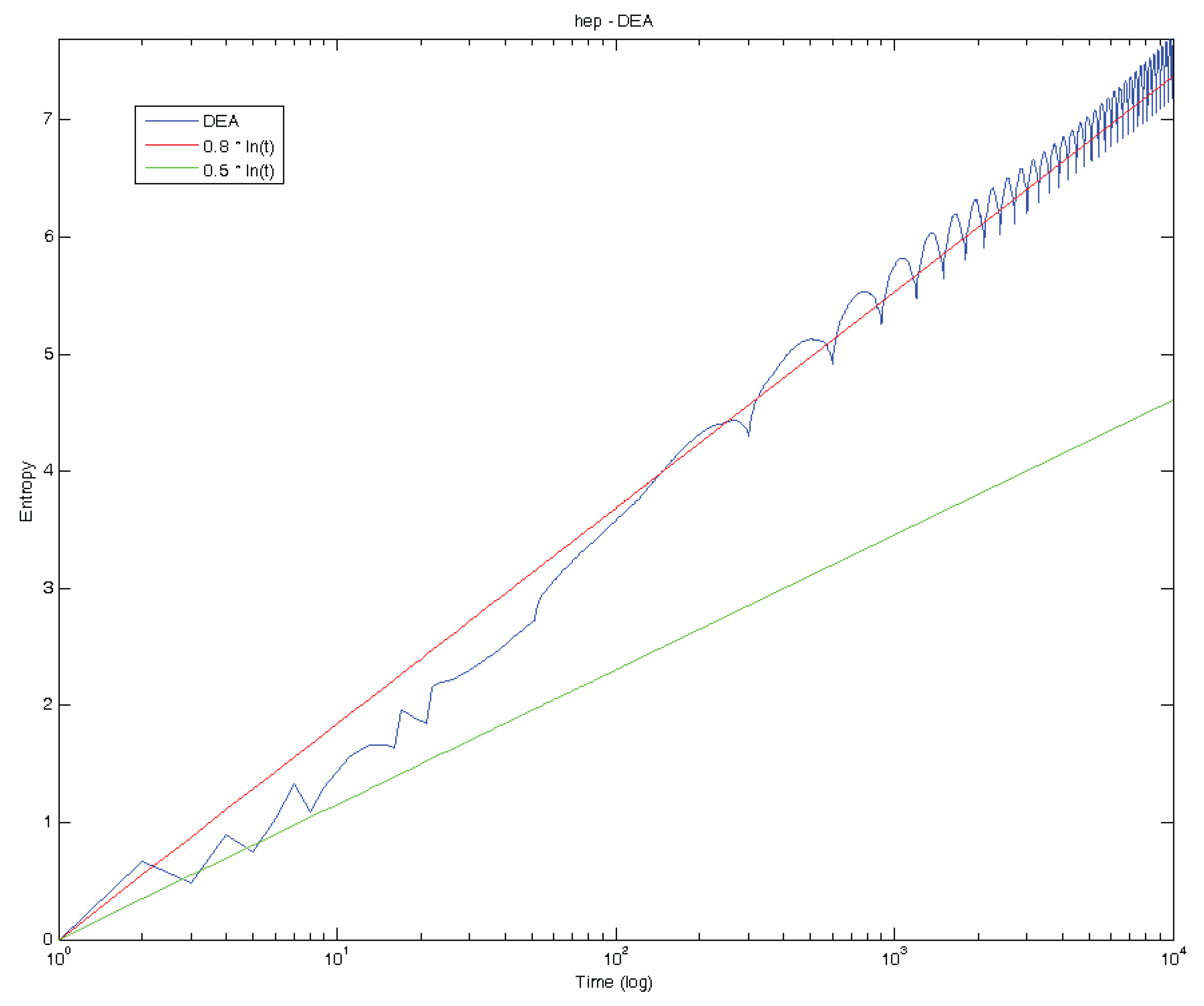
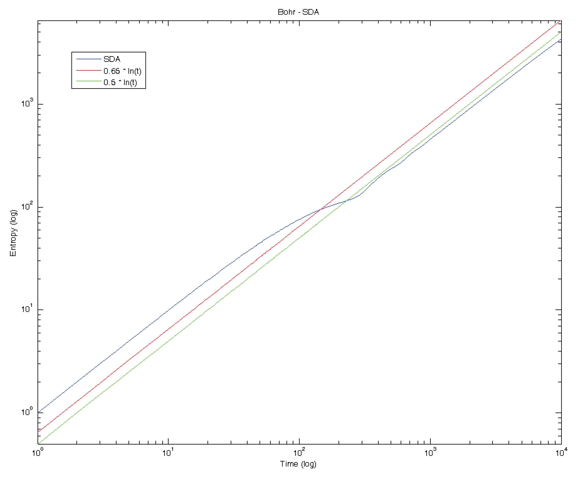
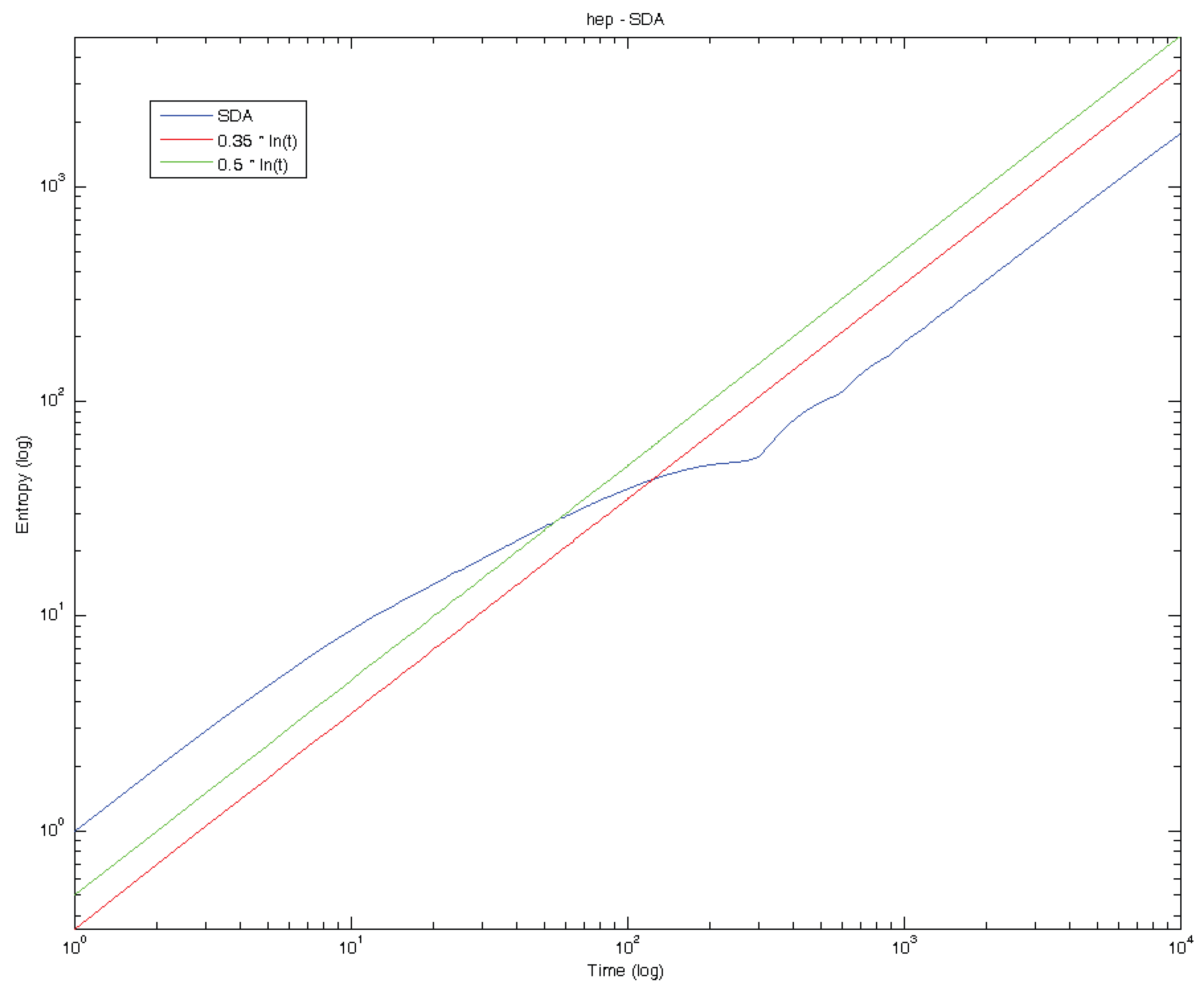
5. Standard Deviation Analysis and Diffusion Entropy Analysis

Scale invariance has been found to hold for complex systems and the correct evaluation of the scaling exponents is of fundamental importance to assess if universality classes exist. Diffusion is typically quantified in terms of a relationship between fluctuation of a variable x and time t. A widely used method of analysis of complexity rests on the assessment of the scaling exponent of the diffusion process generated by a time series. According to the prescription of Peng et al. [15], the numbers of a time series are interpreted as generating diffusion fluctuations and one shifts the attention from the time series to the probability density function (pdf) $p(x,t)$, where x denotes the variable collecting the fluctuations and t is the diffusion time. In this case, if the time series is stationary, the scaling property of the pdf of the diffusion process takes the form

$$p(x,t)=\frac{1}{t^{\delta }}F\left(\frac{x}{t^{\delta }}\right)$$

(5.1)

where δ is a scaling exponent. Diffusion may scale linearly with time, leading to ordinary diffusion, or it may scale nonlinearly with time, leading to anomalous diffusion. Anomalous diffusion processes can be classified as Gaussian or Lévy, depending on whether the central limit theorem (CLT) holds. CLT entails ordinary statistical mechanics. That is, it entails a Gaussian form for F in Equation (5.1) composing a random walk without temporal correlations (i.e., $\delta =0$). Due to the CLT, the probability function $p(x,t)$ describing the probabilities of $x(t)$ has a finite second moment $<x^2>$, and when the second moment diverges, $x(t)$ no longer falls under the CLT and instead indicated that the generalized central limit theorem applies. Failures of CLT mean that instead of statistical mechanics, nonextensive statistical mechanics may be utilized [8,9].

Scafetta and Grigolini [16] established that Diffusion Entropy Analysis (DEA), a method of statistical analysis based on the Shannon entropy (see Equation (1.1)) of the diffusion process, determines the correct scaling exponent δ even when the statistical properties, as well as the dynamic properties, are anomalous. The other methods usually adopted to detect scaling, for example the Standard Deviation Analysis (SDA), are based on the numerical evaluation of the variance. Consequently, these methods detect a power index, denoted H by Mandelbrot [17] in honor of Hurst, which might depart from the scaling δ of Equation (5.1). These variance methods (cf. Fourier analysis and wavelet analysis; see [18,19] produce correct results in the Gaussian case, where $H=\delta$, but fail to detect the correct scaling of the pdf, for example, in the case of Lévy flight, where the variance diverges, or in the case of Lévy walk, where δ and H do not coincide, being related by $\delta =1/(3-2H)$. The case $H=\delta =0.5$ is that of a completely uncorrelated random process. The case $\delta =1$ is that of a completely regular process undergoing ballistic motion. Figure 1, Figure 2, Figure 3 and Figure 4 clearly show that the diffusion entropy development over time for solar neutrinos does neither meet the first nor the latter case. The Shannon entropy, Equation (1.1) for the diffusion process at time t, is defined by

$$S(t)=-\int p(x,t)ln[p(x,t)]dx$$

(5.2)

If the scaling condition of Equation (5.1) holds true, it is easy to prove that

$$S(t)=A+\delta ln(t)$$

(5.3)

where

$$A\equiv -{\int }_{-\infty }^{\infty }dyF(y)ln[F(y)]$$

(5.4)

and $y=x/t^{\delta }$. Numerically, the scaling coefficient δ can be evaluated by using fitting curves with the form Equation (5.3) that on a linear-log scale is a straight line. Even though time series extracted from complex environments may not show a pure scaling behavior as in Equation (5.3) but, instead, patterns with oscillations due to periodicities, one can still observe how diffusion entropy grows linearly with time and one can estimate the diffusion exponent with reasonable accuracy.

Figure 1. Standard Diffusion Analysis of the boron solar neutrino data from SuperKamiokande I and II. The green line coincides with a straight line with the slope $\delta =0.5$. The red line reflects the approximated straight slope of the real data with $\delta =0.65$. The exact result of the SDA is shown by the blue line and indicates a change in the diffusion entropy over time from $\delta >0.5$ to $\delta =0.5$.

Figure 1. Standard Diffusion Analysis of the boron solar neutrino data from SuperKamiokande I and II. The green line coincides with a straight line with the slope $\delta =0.5$. The red line reflects the approximated straight slope of the real data with $\delta =0.65$. The exact result of the SDA is shown by the blue line and indicates a change in the diffusion entropy over time from $\delta >0.5$ to $\delta =0.5$.

Figure 2. Diffusion Entropy Analysis of the boron solar neutrino data from SuperKamiokande I and II. The green line coincides with a straight line with the slope $\delta =0.5$. The red line reflects the approximated straight slope of the real data with $\delta =0.88$. In comparison with Figure 1, the green and red lines are remarkable different from each other and indicate strong anomalous diffusion. The exact result of the DEA is shown by the blue line and indicates a development over time from periodic modulation to asymptotic saturation.

Figure 2. Diffusion Entropy Analysis of the boron solar neutrino data from SuperKamiokande I and II. The green line coincides with a straight line with the slope $\delta =0.5$. The red line reflects the approximated straight slope of the real data with $\delta =0.88$. In comparison with Figure 1, the green and red lines are remarkable different from each other and indicate strong anomalous diffusion. The exact result of the DEA is shown by the blue line and indicates a development over time from periodic modulation to asymptotic saturation.

Figure 3. Standard Diffusion Analysis of the hep solar neutrino data from SuperKamiokande I and II. The green line coincides with a straight line with the slope $\delta =0.5$. The red line reflects the approximated straight slope of the real data with $\delta =0.35$. Note the remarkable difference between the boron analysis results $\delta >0.5$ and the hep analysis results shown in this Figure. with $\delta <0.5$. This is an indication of superdiffusion in the first case and subdiffusion in the second case. The exact result of the SDA is shown by the blue line and indicates a change in the diffusion entropy over time from $\delta >0.5$ to $\delta <0.5$.

Figure 3. Standard Diffusion Analysis of the hep solar neutrino data from SuperKamiokande I and II. The green line coincides with a straight line with the slope $\delta =0.5$. The red line reflects the approximated straight slope of the real data with $\delta =0.35$. Note the remarkable difference between the boron analysis results $\delta >0.5$ and the hep analysis results shown in this Figure. with $\delta <0.5$. This is an indication of superdiffusion in the first case and subdiffusion in the second case. The exact result of the SDA is shown by the blue line and indicates a change in the diffusion entropy over time from $\delta >0.5$ to $\delta <0.5$.

Figure 1, Figure 2, Figure 3 and Figure 4, respectively, are showing diffusion entropy as a function of time for two different time series. Figure 1, Figure 2, Figure 3 and Figure 4 show the numerical results of Standard Deviation Analysis and Diffusion Entropy Analysis for solar neutrino data taken by the SuperKamiokande experiments I (SK-I, 1996–2001, 1496 days, 5.0–20.0 MeV) and II (SK-II, 2002–2005, 791 days, 8.0–20.0 MeV). SuperKamiokande [20] is a 50 kiloton water Cherenkov detector located at the Kamioka Observatory of the Institute for Cosmic Ray Research, University of Tokyo. It was designed to study solar neutrino oscillations and carry out searches for the decay of the nucleon. The SuperKamiokande experiment began in 1996 and in the ensuing decade of running has produced extremely important results in the fields of atmospheric and solar neutrino oscillations, along with setting stringent limits on the decay of the nucleon and the existence of dark matter and astrophysical sources of neutrinos. Perhaps most crucially, Super-Kamiokande for the first time definitely showed that neutrinos have mass and undergo flavor oscillations.

An additional feature of the $S(t)$ behavior over time in Figure 2 and Figure 4 are distinct oscillations characteristic for processes with periodic modulation and asymptotic saturation. They appear for large δ. At the current stage of research the origin of these oscillations is an open problem [21].

Figure 4. Diffusion Entropy Analysis of the hep solar neutrino data from SuperKamiokande I and II. The green line coincides with a straight line with the slope $\delta =0.5$. The red line reflects the approximated straight slope of the real data with $\delta =0.8$. In comparison with Figure 3, the green and red lines are remarkable different from each other similar to the boron data analysis and indicate strong anomalous diffusion. The exact result of the DEA is shown by the blue line and indicates a development over time from periodic modulation to asymptotic saturation similar to the boron analysis results.

Figure 4. Diffusion Entropy Analysis of the hep solar neutrino data from SuperKamiokande I and II. The green line coincides with a straight line with the slope $\delta =0.5$. The red line reflects the approximated straight slope of the real data with $\delta =0.8$. In comparison with Figure 3, the green and red lines are remarkable different from each other similar to the boron data analysis and indicate strong anomalous diffusion. The exact result of the DEA is shown by the blue line and indicates a development over time from periodic modulation to asymptotic saturation similar to the boron analysis results.

6. Conclusions

An α-generalized entropy measure, parallel to Havrda-Charvat entropy and related to Tsallis entropy, for the scalar, multivariable, and matrix case, respectively, was introduced. This entropy measure was optimized under different types of restrictions leading to generalized type-1 beta family of densities, generalized type-2 beta family of densities, and generalized gamma family of densities. The pathway model, through its α parameter, established links between many entropic, distributional and differential models utilized in the literature. The pathway model provides the ways and means to switch from the Gaussian form of densities to heavy-tailed densities, and, through appropriate normalizing constants, to statistical densities. The simplest case in the pathway model, Shannon entropy, is used for the numerical treatment of diffusion entropy analysis and compared to standard deviation analysis for solar neutrino data from SuperKamiokande. Such a procedure will be extended to other entropy measures of the pathway model in the future. Results of evaluating the simplest case, Shannon entropy, already shows that the solar neutrino data show non-Gaussian signature and contain a signal of modulation with subsequent saturation. This is a clear indication of the superiority of diffusion entropy analysis, focusing on the time development of the probability density function, in contrast to standard deviation analysis, focusing on the time development of the variance. Consequences of this results for so-called solar modeling will be discussed elsewhere.

References

1. Greven, A.; Keller, G.; Warnecke, G. Entropy; Princeton University Press: Princeton, NJ, USA, 2003. [Google Scholar]
2. Penrose, R. Cycles of Time: An Extraordinary New View of the Universe; The Bodley Head: London, UK, 2010. [Google Scholar]
3. Mathai, A.M. A pathway to matrix variate gamma and normal densities. Linear Algebra Appl. 2005, 396, 317–328. [Google Scholar] [CrossRef]
4. Tsallis, C. Possible generalizations of Boltzmann-Gibbs statistics. J. Stat. Phys. 1988, 52, 479–487. [Google Scholar] [CrossRef]
5. Beck, C. Stretched exponentials from superstatistics. Physica A 2006, 365, 96–101. [Google Scholar] [CrossRef]
6. Beck, C.; Cohen, E.G.D. Superstatistics. Physica A 2003, 322, 267–275. [Google Scholar] [CrossRef]
7. Mathai, A.M.; Rathie, P.N. Basic Concepts in Information Theory and Statistics: Axiomatic Foundations and Applications; Wiley Eastern: New Delhi, India; Wiley Halsted: New York, NY, USA, 1975. [Google Scholar]
8. Gell-Mann, M.; Tsallis, C. Nonextensive Entropy: Interdisciplinary Applications; Oxford University Press: New York, NY, USA, 2004. [Google Scholar]
9. Tsallis, C. Introduction to Nonextensive Statistical Mechanics: Approaching a Complex World; Springer: New York, NY, USA, 2009. [Google Scholar]
10. Mathai, A.M. Jacobians of Matrix Transformations and Functions of Matrix Argument; World Scientific Publishing: New York, NY, USA, 1997. [Google Scholar]
11. Mathai, A.M. Some properties of Mittag-Leffler functions and matrix-variate analogues: A statistical perspective. Fract. Calc. Appl. Anal. 2010, 13, 113–132. [Google Scholar]
12. Mathai, A.M.; Haubold, H.J. Pathway model, superstatistics, Tsallis statistics and a generalized measure of entropy. Physica A 2007, 375, 110–122. [Google Scholar] [CrossRef]
13. Mathai, A.M.; Haubold, H.J. Special Functions for Applied Scientists; Springer: New York, NY, USA, 2008. [Google Scholar]
14. Mathai, A.M.; Provost, S.B.; Hayakawa, T. Bilinear Forms and Zonal Polynomials; Springer: New York, NY, USA, 1995. [Google Scholar]
15. Peng, C.K.; Buldyrev, S.V.; Havlin, S.; Simons, M.; Stanley, H.E.; Goldberger, A.L. Mosaic organization of DNA nucleotides. Phys. Rev. E 1995, 49, 1685–1689. [Google Scholar] [CrossRef]
16. Scafetta, N.; Grigolini, P. Scaling detection in time series: Diffusion entropy analysis. Phys. Rev. E 2002. [Google Scholar] [CrossRef] [PubMed]
17. Mandelbrot, B.B. The Fractal Geometry of Nature; W.H. Freeman and Company: New York, NY, USA, 1983. [Google Scholar]
18. Haubold, H.J.; Mathai, A.M. A heuristic remark on the periodic variation in the number of solar neutrinos detected on Earth. Astrophys. Space Sci. 1995, 228, 113–134. [Google Scholar] [CrossRef] [Green Version]
19. Sakurai, K.; Haubold, H.J.; Shirai, T. The variation of the solar neutrino fluxes over time in the Homestake, GALLEX(GNO), and the Super-Kamiokande experiments. Space Radiat. 2008, 5, 207–216. [Google Scholar]
20. SuperKamiokande. Available online: http://www-sk.icrr.u-tokyo.ac.jp/sk/index-e.html (accessed on 20 September 2013).
21. Sebastian, N.; Joseph, D.P.; Nair, S.S. Overview of the pathway idea in statistical and physical sciences. arXiv:1307.793 [math-ph].