The Entropy of a Discrete Real Variable

Abstract

The discrete Shannon entropy H was formulated only to measure indeterminacy effected through a set of probabilities, but the indeterminacy in a real-valued discrete variable depends on both the allowed outcomes $\mathbf{x}$ and the corresponding probabilities $\mathbf{p}$. A fundamental measure that is sensitive to both $\mathbf{x}$ and $\mathbf{p}$ is derived here from the total differential entropy of a continuous real variable and its conjugate in the discrete limit, where the conjugate is universally eliminated. The asymptotic differential entropy recovers H plus the new measure, named Ξ, which provides a novel probe of intrinsic organization in sequences of real numbers.

1. Introduction

Let Y be a discrete variable with $n>1$ generic outcomes $\mathbf{y}=\{y_1,\cdots ,y_n\}$ and corresponding probabilities $\mathbf{p}=\{p_1,\cdots ,p_n\}$ such that

$$\sum _{j=1}^n{p}_j=1$$

(1)

Expressed in terms of the natural logarithm, the Shannon entropy attributed to Y in connection with $\mathbf{p}$ is [1]

$$H\left(\mathbf{p}\right)=-\sum _{j=1}^n{p}_j\log \left(p_j\right)$$

(2)

For convenience let

$$H_2\left(\mathbf{p}\right)\equiv \frac{H\left(\mathbf{p}\right)}{\log \left(2\right)}$$

(3)

represent the original form defined in terms of the base-2 logarithm. $H=H\left(\mathbf{p}\right)$ is bound according to

$$0\le H\le \log \left(n\right)$$

(4)

The maximum is generated only when all outcomes are equally probable. $H\left(\mathbf{p}\right)$ vanishes in the limit as some $p_j\in \mathbf{p}$ approaches unity, which represents a completely predetermined outcome.

Because it emerges naturally from the basic principles of encoded compression, the discrete Shannon entropy is widely recognized as an informatic measure. Specifically, consider a message $\mathbf{m}$ consisting of $N\gg 1$ symbols from a generalized alphabet $\mathbf{s}=\{s_1,\cdots ,s_a\}$. Let $N_j$ represent the total number of occurrences of a particular symbol $s_j\in \mathbf{s}$ within $\mathbf{m}$. In the limit as N becomes infinitely large suppose that each $N_j/N$ approaches a certain constant $w_j$ that is characteristic to the “language” in which $\mathbf{m}$ is composed. For sufficiently large N we therefore have $N_j\simeq w_{j}N$. The total number I of likely messages of length N is consequently fixed by $\mathbf{w}=\{w_1,\cdots ,w_a\}$ according to

$$I\simeq \prod _{j=1}^n{w}_j^{-N_j}$$

(5)

The right side of Equation (5) is simply the inverse of the probability for finding any one particular $\mathbf{m}$ among all messages of length N subject to $\mathbf{w}$. The inventory of likely messages could be encoded as I different integers. The number β of bits required to register the encoded inventory is given by $\beta =\lceil {\log }_2\left(I\right)\rceil$, and we therefore have the average compression rate

$$\frac{\beta }{N}\simeq H_2\left(\mathbf{w}\right)$$

(6)

Notwithstanding its significance, Equation (6) represents only a particular example of the expansive utility of the discrete Shannon entropy. Interpreted most broadly, and in accordance with the purpose for which it was derived, $H\left(\mathbf{p}\right)$ measures the indeterminacy in a random selection from among n different options with corresponding probabilities $\mathbf{p}$ [1]. It is therefore appropriate to attribute a quantity of entropy $H\left(\mathbf{p}\right)$ to a discrete variable with probabilities $\mathbf{p}$.

Consider a variable Y whose $n\gg 1$ allowed outcomes $\mathbf{y}$ are governed by some $\mathbf{p}$ such that $H\left(\mathbf{p}\right)$ is near $\log \left(n\right)$. The nearly maximal entropy implies that Y exhibits no significant statistical preference toward any particular outcome or group of outcomes among $\mathbf{y}$. Consequently an ideal observer who studied the behavior of Y could develop a successful model only to predict the most trivial details about future outcomes. Stated alternatively, the degree to which Y behaves deterministically is minimal. In contrast suppose that $H\left(\mathbf{p}\right)$ is much smaller than $\log \left(n\right)$. The nearly minimal entropy implies a strong statistical preference for some comparatively small number of $y_j\in \mathbf{y}$. As such Y would exhibit an appreciable degree of deterministic behavior. A successful, non-trivial predictive model could be therefore developed from observations of Y.

It is important to emphasize that H is a rigorous measure of indeterminacy in a variable only insofar as the indeterminacy depends on $\mathbf{p}$ alone. Let X be a discrete variable whose n allowed outcomes $\mathbf{x}=\{x_1,\cdots ,x_n\}$ are D-dimensional real vectors, i.e. $x_j\in {\Re }^{\mathit{D}}$ for $j=1,\cdots ,n$. The elements of every one-dimensional $\mathbf{x}$ are implicitly listed in ascending order throughout the following. Analogously to the real nature of $\mathbf{p}$, the real nature of $\mathbf{x}$ endows the outcomes of X with definite spatial attributes in which non-trivial deterministic behaviors could manifest. Consequently, as illustrated in the following two examples, H is not generally sufficient as a measure of indeterminacy in real-valued discrete variables.

Consider two variables $X_{ee}$ and $X_{er}$ whose outcomes are confined to the real axis. Let the allowed outcomes of $X_{ee}$ be equally probable and equally spaced, hence the subscript “$ee$”, and let the allowed outcomes of $X_{er}$ be equally probable but randomly spaced, hence the subscript “$er$”. More formally, the allowed outcomes of $X_{ee}$ are of the form ${\mathbf{x}}_e$, which is defined for $D=1$ to be a set of n equally spaced points on the real axis. Let γ represent the arbitrary spacing in a given ${\mathbf{x}}_e$. For convenience we also define ${\mathbf{p}}_e\equiv \{1/n,\cdots ,1/n\}$ for a given n to represent a set of equal probabilities. The allowed outcomes of $X_{er}$ are of the form ${\mathbf{x}}_r$, which is defined for $D=1$ to be indistinguishable from a set of n points distributed randomly over some simple finite segment ${\mathfrak{X}}_1$ of the real axis. The intrinsic spatial structure of ${\mathbf{x}}_e$ effects a commensurate degree of deterministic behavior in $X_{ee}$. For instance, the difference between successive outcomes of $X_{ee}$ is always an integer multiple of γ, and is therefore significantly more predictable than the difference between successive outcomes of $X_{er}$. Because $X_{ee}$ and $X_{er}$ differ only in the spatial arrangement of their allowed outcomes, $X_{ee}$ would behave more deterministically. By definition a smaller quantity of entropy should be therefore attributed to $X_{ee}$. The discrete Shannon entropy attributed to both variables, however, would be identically maximal.

Consider next a complementary scenario in which the allowed outcomes are identically valued but the respective probabilities differ. Let $X_{re}$ and $X_{ae}$ be two variables with $n\gg 1$ one-dimensional allowed outcomes of the form ${\mathbf{x}}_e$. The set of probabilities governing $X_{re}$ is of the form ${\mathbf{p}}_r$, which is defined generally to be indistinguishable from n randomly selected positive real numbers, subsequently normalized to unity and listed in random order. The spatial assignment of ${\mathbf{p}}_r$ through ${\mathbf{x}}_e$ would be globally isotropic but locally irregular, despite the intrinsic structure of ${\mathbf{x}}_e$. The outcomes of $X_{ae}$ are matched to a set of probabilities of the form ${\mathbf{p}}_a$, which is defined generally to be indistinguishable from n randomly selected positive real numbers, subsequently normalized to unity and listed in ascending order. The ordered arrangement of ${\mathbf{p}}_a$ effects a non-trivial deterministic bias favoring progressively larger outcomes in $X_{ae}$. Note that the specific form of ${\mathbf{p}}_a$ in this example could be constructed simply by sorting the elements of ${\mathbf{p}}_r$, in which case $X_{ae}$ would behave more deterministically but $H\left({\mathbf{p}}_r\right)$ and $H\left({\mathbf{p}}_a\right)$ would be identical.

The problems raised in the previous two paragraphs do not imply any flaw in H. The discrete Shannon entropy was formulated only to measure indeterminacy effected by a given $\mathbf{p}$ in a generic discrete variable. The net indeterminacy in a real-valued discrete variable, however, depends on the respective intrinsic characteristics of $\mathbf{x}$ and $\mathbf{p}$, and on the manner in which $\mathbf{x}$ and $\mathbf{p}$ are matched. A special measure is therefore required for discrete real variables. Note that Equation (6) is insensitive to the nature of $\mathbf{s}$, and the present considerations are therefore irrelevant in the context of the coding theorems. To be precise, the role of $H_2$ in Equation (6) is not truly as a measure of indeterminacy.

Although it included no special provisions for discrete real variables, Shannon’s seminal paper introduced a separate formulation for the entropy of a continuous real variable. Let $\mathcal{X}$ be a probabilistically determined variable whose allowed outcomes span a continuum of real vectors within some region $\mathfrak{X}\in {\Re }^{\mathit{D}}$. Let the probability density $\rho \left(x\right)$ be defined such that $\rho \left(x\right)\mathrm{d}x$ gives the probability for an outcome of $\mathcal{X}$ to lie within an infinitesimal element $\mathrm{d}x$ centered on x, where $x\in {\Re }^{\mathit{D}}$ is an independent variable and $\mathrm{d}x=\mathrm{d}{x}^{\left(1\right)}\cdots \mathrm{d}{x}^{\left(D\right)}$ represents implicitly the product of the differentials of each vector component of $x=(x^{\left(1\right)},\cdots ,x^{\left(D\right)})$. We therefore require $\rho =\rho \left(x\right)$ to vanish for all $x\notin \mathfrak{X}$. The normalization of ρ is accordingly

$$\underset{{\Re }^{\mathit{D}}}{\int }\rho \mathrm{d}x=\underset{\mathfrak{X}}{\int }\rho \mathrm{d}x=1$$

(7)

Henceforth any integration is understood to span ${\Re }^{\mathit{D}}$ in the absence of explicit limits. The entropy $\mathcal{H}=\mathcal{H}\left(\rho \right)$ attributed to $\mathcal{X}$ in connection with ρ is [1]

$$\mathcal{H}=-\int \rho \log \left(\rho \right)\mathrm{d}x$$

(8)

where $\rho \log \left(\rho \right)$ is defined to vanish for $\rho =0$. The measure in Equation (8) is known as the differential (Shannon) entropy.

In contrast to H a single quantity of $\mathcal{H}$ is subject to no finite bounds. Consequently a simple comparison between H and $\mathcal{H}$ is not meaningful. For instance, the differential entropy of a normalized Gaussian

$${\rho }_{\mathit{G}}={\rho }_{\mathit{G}}(\nu ,x)\equiv {\left(\frac{\nu }{\sqrt{\pi }}\right)}^D{e}^{-{\nu }^2{x}^2}$$

(9)

is $D\log (\sqrt{\pi e}/\nu )$. For ν equal to $\sqrt{\pi e}$ the entropy vanishes, which signifies a predetermined outcome in the context of discrete real variables. Furthermore in the limit as ν becomes infinitely large ${\rho }_{\mathit{G}}$ behaves as a D-dimensional delta-distribution $\delta \left(x\right)$, which describes a single predetermined real outcome. $\mathcal{H}\left({\rho }_{\mathit{G}}\right)$, however, decreases without bound as ν approaches infinity.

The apparent inconsistencies between H and $\mathcal{H}$ are reconciled in the following manner. As a generalization of ${\rho }_{\mathit{G}}$ let ${\rho }_0={\rho }_0(\nu ,x)$ be some well-behaved, unity-normalized function that becomes $\delta \left(x\right)$ in the limit as the positive, real parameter ν becomes infinitely large. In association with an arbitrary X, with n allowed outcomes $\mathbf{x}$ and corresponding probabilities $\mathbf{p}$, let the probability density ${\rho }_{\mathit{X}}={\rho }_{\mathit{X}}(\nu ,x)$ be defined such that

$${\rho }_{\mathit{X}}(\nu ,x)\sim B\sum _{j=1}^n{p}_j{\rho }_0(\nu ,x-x_j)$$

(10)

and thus

$$\underset{\nu \to \infty }{lim}{\rho }_{\mathit{X}}=\sum _{j=1}^n{p}_j\delta (x-x_j)$$

(11)

where $B=B\left(\nu \right)$ is the appropriate normalization coefficient for a given ν, and $x_j$ and $p_j$ span $\mathbf{x}$ and $\mathbf{p}$ respectively. The symbol “∼” is used in Equation (10) and throughout, where convenient, to signify asymptotic equality as ν approaches infinity. The right side of Equation (11) describes the probabilistic behavior of X. Consider an originally continuous test variable ${\mathcal{X}}_{\mathit{X}}$ whose outcomes are governed by ${\rho }_{\mathit{X}}$. The entropy attributed to ${\mathcal{X}}_{\mathit{X}}$ is $\mathcal{H}\left({\rho }_{\mathit{X}}\right)$, which behaves asymptotically as

$$\mathcal{H}\left({\rho }_{\mathit{X}}\right)\sim -B\sum _{j=1}^n{p}_j\int {\rho }_0\log \left(B{p}_j{\rho }_0\right)\mathrm{d}x$$

(12)

When ν is finite but very large the behavior of ${\mathcal{X}}_{\mathit{X}}$ is a hybrid of the continuous traits of ${\rho }_0$ and the discrete traits of $\mathbf{x}$ and $\mathbf{p}$. In the limit as $\nu \to \infty$ the two sets of traits become completely disassociated from one another, and ${\mathcal{X}}_{\mathit{X}}=X$ is characterized only by $\mathbf{x}$ and $\mathbf{p}$. The entropy associated with the probabilistic behavior of X should be therefore given by the asymptote of $\mathcal{H}\left({\rho }_{\mathit{X}}\right)-\mathcal{H}\left({\rho }_0\right)$. From Equation (12) we readily obtain

$$\underset{\nu \to \infty }{lim}\left(\mathcal{H}\left({\rho }_{\mathit{X}}\right)-\mathcal{H}\left({\rho }_0\right)\right)=-\sum _{j=1}^n{p}_j\log \left(p_j\right)$$

(13)

thereby recovering H from $\mathcal{H}$.

Although the analysis leading to Equation (13) may be instructive, $\mathcal{H}\left({\rho }_{\mathit{X}}\right)$ is asymptotically independent of $\mathbf{x}$ and could not produce the desired new measure for discrete real variables. It is reasonable to suspect that some additional quantity of the form $\mathcal{H}$ could be considered in conjunction with $\mathcal{H}\left({\rho }_{\mathit{X}}\right)$ to provide the required asymptotic sensitivity to both $\mathbf{x}$ and $\mathbf{p}$. In order to be meaningful, however, the additional measure should be intrinsically related to ${\rho }_{\mathit{X}}$.

Within the paradigm of wave mechanics two distinct quantities of differential entropy are naturally associated with a given ρ. More precisely, two separate probability density functions are naturally associated with a given probability amplitude $\psi =\psi \left(x\right)$, namely $\rho ={\left|\psi \right|}^2$ and the spectral density

$$\widehat{\rho }\left(k\right)={\left|\widehat{\psi }\left(k\right)\right|}^2$$

(14)

where

$$\widehat{\psi }=\widehat{\psi }\left(k\right)={\left(\frac{1}{\sqrt{2\pi }}\right)}^D\int \psi e^{-ik·x}\mathrm{d}x$$

(15)

is the Fourier-conjugate of ψ and $k\in {\Re }^{\mathit{D}}$ is an independent variable. We may interpret $\widehat{\rho }=\widehat{\rho }\left(k\right)$ as the probability density governing the outcomes of a variable $\mathcal{K}$ that is the conjugate of the variable $\mathcal{X}$ governed by ρ. The entropy attributed to $\mathcal{K}$ in connection with $\widehat{\rho }$ is $\mathcal{H}\left(\widehat{\rho }\right)$. The total differential entropy attributed to the conjugated pair is therefore

$$S\left(\psi \right)\equiv {\mathcal{H}\left(\right|\psi |}^2)+\mathcal{H}(|\widehat{\psi }{|}^2)$$

(16)

A more formal derivation of $S=S\left(\psi \right)$ follows from the total phase-space distribution [9]

$$f=f(x,k)\equiv \rho \widehat{\rho }$$

(17)

which is subject to the normalization

$$\int f\mathrm{d}r=1,$$

(18)

where $r\equiv \left(x^{\left(1\right)},\cdots ,x^{\left(D\right)},k^{\left(1\right)},\cdots ,k^{\left(D\right)}\right)$ for any given x and k. Because f is simply a probability density in a $2D$-dimensional vector space, it is appropriate to attribute a quantity of differential entropy

$$-\int f\log \left(f\right)\mathrm{d}r=S$$

(19)

to the conjugated pair.

The total differential entropy S has been the subject of extensive research. (See, for instance, [2,3,4,5,6,7,8]). It is worthwhile to mention here two general characteristics that distinguish S as a fundamentally important measure. Because f is dimensionless S, like the relative entropy, is free from a potentially serious flaw to which the differential Shannon entropy is otherwise vulnerable [10]. Furthermore, whereas $\mathcal{H}\left(\rho \right)$ and $\mathcal{H}\left(\widehat{\rho }\right)$ may become infinitely negative, S is subject to the lower bound [2]

$$S\ge D\log \left(\pi e\right)$$

(20)

Perhaps uniquely, a Gaussian amplitude generates the minimal S allowed by Equation (20) [2].

The purpose of this article is to demonstrate that a measure of indeterminacy for discrete real variables that is sensitive to both $\mathbf{x}$ and $\mathbf{p}$ emerges from the total differential entropy of ${\mathcal{X}}_{\mathit{X}}$ and its conjugate in the limit as ν diverges. Specifically, the conjugated analogue of Equation (13) includes an additional measure $\Xi =\Xi (\mathbf{p},\mathbf{x})$, expressed most generally in terms of an integral, that behaves naturally as a measure of indeterminacy in the spatial configuration of $\mathbf{x}$ and $\mathbf{p}$. Furthermore the conjugate is universally eliminated in the limit as ${\mathcal{X}}_{\mathit{X}}$ becomes discrete and the entire residual entropy $H+\Xi$, named η is therefore attributed to X. Section 2 contains a derivation of η. The general characteristics of η are examined in Section 3. Section 4 presents a quantitative study demonstrating the basic behaviors of η as a measure of indeterminacy for discrete real variables. The primary conclusions are summarized and interpreted in Section 5.

2. Derivation of η

The terms defined in Section 1 retain their definitions throughout the following. Let ${\mathcal{K}}_{\mathit{X}}$ be the conjugate of a given ${\mathcal{X}}_{\mathit{X}}$. The probability density ${\widehat{\rho }}_{\mathit{X}}={\widehat{\rho }}_{\mathit{X}}(\nu ,k)$ governing the outcomes of ${\mathcal{K}}_{\mathit{X}}$ is formulated presently. Let ${\psi }_{\mathit{X}}={\psi }_{\mathit{X}}(\nu ,x)$ be defined such that ${\rho }_{\mathit{X}}={\left|{\psi }_{\mathit{X}}\right|}^2$. The total differential entropy of the conjugated pair is thus $S\left({\psi }_{\mathit{X}}\right)=\mathcal{H}\left({\rho }_{\mathit{X}}\right)+\mathcal{H}\left({\widehat{\rho }}_{\mathit{X}}\right)$. This section contains a derivation of the asymptotic form of $S\left({\psi }_{\mathit{X}}\right)$ expressed analogously to Equation (13).

The first step is to formulate ${\psi }_{\mathit{X}}$. Following the standard wave-mechanical prescription, and in accordance with natural law, we attribute to each allowed outcome a separate amplitude [11]. The total amplitude is simply the sum of the individual amplitude waveforms multiplied by an appropriate normalization coefficient. Let the probability amplitude ${\varphi }_0={\varphi }_0(\nu ,x)$ be therefore defined such that $|{\varphi }_0{|}^2={\rho }_0$, i.e.,

$$\underset{\nu \to \infty }{lim}|{\varphi }_0{|}^2=\delta \left(x\right)$$

(21)

The waveform assigned to each $x_j\in \mathbf{x}$ is

$${\varphi }_j={\varphi }_j(\nu ,x)\equiv \sqrt{p_j}{\varphi }_0(\nu ,x-x_j)$$

(22)

and the total amplitude is accordingly

$${\psi }_{\mathit{X}}=A\sum _{j=1}^n{\varphi }_j$$

(23)

where $A=A\left(\nu \right)$ is defined such that ${\rho }_{\mathit{X}}$ is unity-normalized for all ν. Because the real part of ${\varphi }_0$ becomes ever more sharply peaked with increasing ν, the cross terms ${\left|A\right|}^2{\varphi }_j{\varphi }_l^{*}$ in $|{\psi }_{\mathit{X}}{|}^2$ are negligible for sufficiently large ν and vanish asymptotically. We therefore have

$${\rho }_{\mathit{X}}\sim {\left|A\right|}^2\sum _{j=1}^n|{\varphi }_j{|}^2$$

(24)

which is equivalent to Equation (10). Note that

$$\underset{\nu \to \infty }{lim}{\left|A\right|}^2=\underset{\nu \to \infty }{lim}B=1$$

(25)

The next step is to determine the respective forms of the conjugate amplitude ${\widehat{\psi }}_{\mathit{X}}={\widehat{\psi }}_{\mathit{X}}(\nu ,k)$ and density ${\widehat{\rho }}_{\mathit{X}}={\left|{\widehat{\psi }}_{\mathit{X}}\right|}^2$. Let ${\widehat{\varphi }}_0={\widehat{\varphi }}_0(\nu ,k)$ represent the conjugate of ${\varphi }_0$, and let the associated density $|{\widehat{\varphi }}_0{|}^2$ be defined as ${\widehat{\rho }}_0={\widehat{\rho }}_0(\nu ,k)$. It follows from Equation (15), with $x-x_j$ substituted for x, that

$${\widehat{\varphi }}_j=\sqrt{p_j}{e}^{-ık·x_j}{\widehat{\varphi }}_0$$

(26)

where ${\widehat{\varphi }}_j={\widehat{\varphi }}_j(\nu ,k)$ is the conjugate of a given ${\varphi }_j$. We therefore have

$${\widehat{\psi }}_{\mathit{X}}=A{\widehat{\varphi }}_0\sum _{j=1}^n\sqrt{p_j}{e}^{-ık·x_j}$$

(27)

and thus

$${\widehat{\rho }}_{\mathit{X}}={\left|A\right|}^2\tau {\widehat{\rho }}_0$$

(28)

where

$$\tau \equiv {\left|\sum _{j=1}^n\sqrt{p_j}{e}^{-ık·x_j}\right|}^2$$

(29)

An equivalent expression for $\tau =\tau \left(k\right)$ following from the Euler identity is

$$\tau =1+2\sum _{j=1}^{n-1}\left\{\sum _{l=j+1}^n\sqrt{p_j{p}_l}cos\left((x_l-x_j)·k\right)\right\}$$

(30)

For convenience we define $\zeta =\zeta \left(k\right)$ such that $\tau =1+2\zeta$.

The asymptotic behavior of ${\widehat{\rho }}_{\mathit{X}}$ is ascertained readily from the explicit form of ${\widehat{\varphi }}_0$ in Equation (15) with ${\varphi }_0$ expressed as ${\rho }_0/{\varphi }_0^{*}$ for all non-vanishing ${\varphi }_0^{*}$. It follows from the behavior ascribed to ${\rho }_0$ that

$${\widehat{\varphi }}_0\sim {\left(\frac{1}{\sqrt{2\pi }}\right)}^D\frac{1}{{\varphi }_0^{*}\left(0\right)}$$

(31)

which is independent of k. Because $\int {\rho }_0\mathrm{d}k$ must remain unity-normalized ${\widehat{\varphi }}_0$ must vanish everywhere asymptotically. As ${\rho }_0$ increasingly resembles $\delta \left(x\right)$ the real part of ${\varphi }_0^{*}\left(0\right)$ must either increase or decrease without bound, which ensures that the right side of Equation (31) vanishes. Consequently ${\widehat{\psi }}_{\mathit{X}}$ and ${\widehat{\rho }}_{\mathit{X}}$ vanish asymptotically for all k.

It is also worthwhile to note that, because ${\widehat{\rho }}_{\mathit{X}}$ and ${\widehat{\rho }}_0$ are both unity-normalized for all ν, Equations (28) and (30) imply

$$\underset{\nu \to \infty }{lim}{〈\zeta 〉}_0=0$$

(32)

where

$${〈\epsilon 〉}_0\equiv \int {\widehat{\rho }}_0\epsilon \mathrm{d}k$$

(33)

is the expected value of any $\epsilon =\epsilon \left(k\right)$ averaged against ${\widehat{\rho }}_0$. Equation (32) may be understood as a consequence of the asymptotic uniformity of ${\widehat{\rho }}_0$ in conjunction with the usual trigonometric property

$$\underset{b\to \infty }{lim}{\int }_{-b}^{b}cos\left(k\right)\mathrm{d}k=0$$

(34)

In the limit as ν diverges ${〈\zeta 〉}_0$ becomes simply the average of ζ over all space, which we denote by $\overline{\zeta }$, and thus vanishes term-by-term in accordance with Equation (34). Expressed more generally,

$$\underset{\nu \to \infty }{lim}{〈\epsilon 〉}_0=\overline{\epsilon }.$$

(35)

Returning to the derivation proper, the next step is to evaluate $\mathcal{H}\left({\widehat{\rho }}_{\mathit{X}}\right)$ in the limit as ν approaches infinity. It follows from Equations (25) and (28) that

$$\mathcal{H}\left({\widehat{\rho }}_{\mathit{X}}\right)\sim -{〈\tau \log \left({\widehat{\rho }}_0\right)〉}_0-{〈\tau \log \left(\tau \right)〉}_0$$

(36)

Substituting $1+2\zeta$ for τ in the left-most term on the right side of Equation (36) produces

$$\mathcal{H}\left({\widehat{\rho }}_{\mathit{X}}\right)\sim \mathcal{H}\left({\widehat{\rho }}_0\right)-2{〈\zeta \log \left({\widehat{\rho }}_0\right)〉}_0-{〈\tau \log \left(\tau \right)〉}_0$$

(37)

Although $\log \left({\widehat{\rho }}_0\right)$ decreases without bound it does so with asymptotic uniformity, hence

$${〈\zeta \log \left({\widehat{\rho }}_0\right)〉}_0\sim {〈\zeta 〉}_0\log \left({\widehat{\rho }}_0\left(k_0\right)\right)$$

(38)

for any $k_0\in {\Re }^{\mathit{D}}$. The middle term on the right side of Equation (37) is therefore asymptotically proportional to $\overline{\zeta }$ and thus vanishes. Equation (37) accordingly becomes

$$\mathcal{H}\left({\widehat{\rho }}_{\mathit{X}}\right)\sim \mathcal{H}\left({\widehat{\rho }}_0\right)-{〈\tau \log \left(\tau \right)〉}_0$$

(39)

The asymptotic form of the right-most term in Equation (39) is

$$\Xi (\mathbf{p},\mathbf{x})\equiv -\overline{\tau \log \left(\tau \right)}$$

(40)

Because τ is periodic $\Xi =\Xi (\mathbf{p},\mathbf{x})$ is identical to the average value of $-\tau \log \left(\tau \right)$ taken over some finite region ${\mathfrak{K}}_0\in {\Re }^{\mathit{D}}$ spanning one period in each dimension. We therefore have

$$\Xi =-\frac{1}{{\kappa }_0}\underset{{\mathfrak{K}}_0}{\int }\tau \log \left(\tau \right)\mathrm{d}k$$

(41)

where

$${\kappa }_0\equiv \underset{{\mathfrak{K}}_0}{\int }\mathrm{d}k$$

(42)

An analytical expression for $\int \tau \log \left(\tau \right)\mathrm{d}k$ is possible only for a few rudimentary configurations of $\mathbf{x}$ and $\mathbf{p}$, and Equation (41) is thus critical for quantifying Ξ.

Finally, Equation (39) may be expressed in terms of a proper limit as

$$\underset{\nu \to \infty }{lim}\left(\mathcal{H}\left({\widehat{\rho }}_{\mathit{X}}\right)-\mathcal{H}\left({\widehat{\rho }}_0\right)\right)=\Xi$$

(43)

analogously to Equation (13). Combining Equations (13) and (43) produces the central result

$$\underset{\nu \to \infty }{lim}\left(S\left({\psi }_{\mathit{X}}\right)-S\left({\varphi }_0\right)\right)=\mathbf{p},\mathbf{x})$$

(44)

where

$$\mathbf{p},\mathbf{x})\equiv H(\mathbf{p})+\Xi (\mathbf{p},\mathbf{x})$$

(45)

The nature and behavior of $\mathbf{p},\mathbf{x})$ are examined in the following Sections.

3. General Characteristics of η

By definition $S\left({\psi }_{\mathit{X}}\right)$ measures the net indeterminacy in the conjugated pair ${\mathcal{X}}_{\mathit{X}}$ and ${\mathcal{K}}_{\mathit{X}}$. In the limit as ν becomes infinitely large, however, the pair is characterized completely by $\mathbf{x}$ and $\mathbf{p}$, independently of ${\varphi }_0$. The entropy attributed asymptotically to the pair is therefore η. Furthermore as ${\mathcal{X}}_x$ becomes discrete ${\hat{\rho }}_x$ vanishes everywhere and ${\mathcal{K}}_x$ becomes therefore a “ghost” variable, doomed to exist without ever generating an outcome. The indeterminacy measured by η must be therefore evident in the probabilistic behaviors of X. Because X and its ghost conjugate together are indistinguishable from X alone we conclude that η is a generally valid measure of indeterminacy in discrete real variables.

Given that Ξ is the asymptotic form of $\mathcal{H}\left({\widehat{\rho }}_{\mathit{X}}\right)-\mathcal{H}\left({\widehat{\rho }}_0\right)$ its attribution to X is perhaps counterintuitive, despite the elimination of the conjugate. In particular $\mathcal{H}\left(\rho \right)$ and $\mathcal{H}\left(\widehat{\rho }\right)$ are typically anti-correlated among different ρ of a given generalized form. Recall, however, that $\mathcal{H}\left({\rho }_{\mathit{X}}\right)$ is asymptotically insensitive to $\mathbf{x}$ and therefore is not generally correlated to $\mathcal{H}\left({\widehat{\rho }}_{\mathit{X}}\right)$ in any appreciable manner among different ${\rho }_{\mathit{X}}$. Not only is $\mathcal{H}\left({\widehat{\rho }}_{\mathit{X}}\right)$ sensitive to both $\mathbf{x}$ and $\mathbf{p}$, it is also naturally correlated to the intrinsic indeterminacy effected by the definite spatial attributes of $\mathbf{x}$. Stated most generally, greater spatial regularity in the configuration of $\mathbf{x}$ and $\mathbf{p}$ effects greater harmonic regularity in the spatial arrangement of the peaks in ${\rho }_{\mathit{X}}$, for $\nu \gg 1$. Greater harmonic regularity in ${\rho }_{\mathit{X}}$ implies greater localization in the associated Fourier spectrum, which accordingly generates a smaller $\mathcal{H}\left({\widehat{\rho }}_{\mathit{X}}\right)$, for a given ${\varphi }_0$. In order to isolate the effects associated with $\mathbf{x}$ and $\mathbf{p}$ we exclude the contribution from $\mathcal{H}\left({\widehat{\rho }}_0\right)$. In that manner Ξ measures the deterministic effects of real allowed outcomes.

Lower bounds on η and Ξ follow directly from the universal lower bound on S. Specifically, both $S\left({\psi }_x\right)$ and $S\left({\psi }_0\right)$ are subject to Equation (20) for all ν. We therefore have

$$\eta \ge 0$$

(46)

and thus

$$\Xi \ge -H$$

(47)

Regardless of the degree of spatial structure in the configuration of $\mathbf{x}$ and $\mathbf{p}$, no variable could behave more deterministically than a fixed real number. Equation (46) is therefore consistent with the attribution of zero entropy to a predetermined outcome.

Upper bounds on η and Ξ may be obtained by writing Equation (41) as

$$\Xi =-\underset{{\mathcal{k}}_0}{\int }\frac{\tau }{{𝜅}_0}\log (\frac{\tau }{{𝜅}_0})\text{d}k-\log ({𝜅}_0)$$

(48)

where the right-most term has been reduced using

$$\stackrel{\_}{\tau }=\frac{1}{{𝜅}_0}\underset{{\mathcal{k}}_0}{\int }\tau \text{d}k=1,$$

(49)

which is a consequence of Equation (34). The integral on the right side of Equation (48) is simply the differential Shannon entropy associated with a normalized density τ/k₀ defined over ${\mathcal{K}}_0$. Furthermore log(k₀) is the maximal differential Shannon entropy that could be associated with ${\mathcal{K}}_0$. Equation (48) therefore implies

$$\Xi \le 0$$

(50)

hence

$$\eta \le H$$

(51)

The upper bound on η is consistent with the basic expectations about the predictive utility of real outcomes. Consider some X that has been “disguised” by mapping the n allowed outcomes in $\mathbf{x}$ to a set of n generic outcomes, while keeping the corresponding probabilities $\mathbf{p}$ fixed. An ideal observer who studied only the generic outcomes could form a predictive model only to the extent allowed by $\mathbf{p}$. Suppose that such an observer were subsequently allowed to study the real outcomes. The numeric details could never detract from the observer’s capability to develop a predictive model because, at very least, the outcomes from any $\mathbf{x}$ could be interpreted simply as non-numeric symbols. The entropy attributed to X, therefore, should not be greater than the entropy attributed to the generic analogue, which is precisely what Equation (51) ensures.

For any $\mathbf{p}$, H and η should be similar when the degree of deterministic structure within $\mathbf{x}$ is negligible. We therefore expect

$$\eta (\mathbf{p},{\text{x}}_r)\simeq H\left(\mathbf{p}\right)$$

(52)

which is validated in the following section. Among variables with spatially randomized outcomes, indeterminacy depends primarily on the intrinsic characteristics of $\mathbf{p}$, hence Equation (52). Conversely, among variables with equally probable outcomes, indeterminacy depends only on x. In that manner η($\mathbf{p}$_e, x) measures the intrinsic indeterminacy in the spatial configuration of x. It is therefore fitting, as explicitly evident in Equation (30), that τ is sensitive to each of the n(n − 1)/2 uniquely defined positive intervals x_l − x_j within a given x.

Because there is no preferred region within ${\Re }^{\mathit{D}}$, any meaningful measure of indeterminacy for discrete real variables must be invariant under spatial transformations of the form $\mathbf{x}+\Delta x\equiv \{x_1+\Delta x,\cdots ,x_n+\Delta x\}$ for any finite $\Delta x\in {\Re }^{\mathit{D}}$. By inspecting either Equation (29) or Equation (30) we readily find that τ is translationally invariant, hence

$$\mathbf{p},\mathbf{x}+\Delta x)=\mathbf{p},\mathbf{x})$$

(53)

Similarly transformations of the form $\mathbf{R}\mathbf{x}\equiv \{\mathbf{R}{x}_1,\cdots ,\mathbf{R}{x}_n\}$, where $\mathbf{R}$ is a D-dimensional unitary rotation matrix, could not change the indeterminacy in any X. Consequently the entropy attributed to X must be rotationally invariant as well. The effects of such a rotation would be equivalent to replacing the original $\tau \left(k\right)$ with ${\tau }^{\prime }\left(k\right)=\tau \left(k\mathbf{R}\right)$, which we may write as ${\tau }^{\prime }\left(k\right)=\tau \left(k^{\prime }\right)$ after the variable substitution $k^{\prime }=k\mathbf{R}$. The rotation therefore amounts to nothing more than a cosmetic change of variables, which does not affect the average value of $\tau \log \left(\tau \right)$—whether taken over all space or taken over a finite region spanning a period in each dimension of $k^{\prime }$. We therefore have

$$\eta (\mathbf{p},\mathbf{R}\mathbf{x})=\mathbf{p},\mathbf{x})$$

(54)

For the same reasons we also have

$$\eta (\mathbf{p},\alpha \mathbf{x})=\mathbf{p},\mathbf{x})$$

(55)

for any non-vanishing $\alpha \in \Re$, where $\alpha \mathbf{x}\equiv \{\alpha x_1,\cdots ,\alpha x_n\}$. Contrary to Equation (55), suppose that the entropy of a real discrete variable were to increase under transformations of the form $\alpha \mathbf{x}$ for $\left|\alpha \right|>1$. Consider applying such transformations successively to the allowed outcomes of some non-trivial X. Given that the entropy must never exceed H the effects of the transformations must become negligible at some point, which would imply the existence of some preferred spatial scale for a given $\mathbf{x}$ and $\mathbf{p}$. The indeterminacy, however, could not be sensitive to such a scale. The scale-invariance expressed in Equation (55) is therefore necessary for any meaningful measure of indeterminacy in discrete real variables.

4. Quantitative Study

This section presents the results of numerical calculations of η chosen to validate the identification of η as the entropy of a discrete real variable and to demonstrate the utility of Ξ as a probe of deterministic structure in sequences of real numbers or non-numeric symbols. For convenience this introductory study is restricted to scenarios where $D=1$; the conclusions are readily generalized to higher-dimensional spaces. In each calculation of η reported here the period-averaged value of −τlog(τ) was obtained from 2⁵ ⌊ κ₀/κ_*⌋ samples, where κ_* = 2 π/(x_n − x₁) represents the finest periodicity in τ. Note that x_n − x₁ is always the largest positive interval within a one-dimensional x. All computations were precise to 15 significant figures. The accuracy, in comparison to the “true” value of η produced by an infinite number of samples, is always better than ${10}^{-6}.$η.

The first sets of calculations examined below involve the basic types of $\mathbf{x}$ and $\mathbf{p}$ introduced in Section 1, matched in various instructive combinations. Each ${\mathbf{p}}_r$ was constructed from n different real numbers with 15 significant figures selected randomly from $(0,1)$, and subsequently normalized. Each ${\mathbf{x}}_r$ was constructed by randomly selecting n different integers from $[1,100n]$. This produces approximately the same effect as using the full range available with 15 significant figures, but dramatically reduces processing requirements. For each calculation involving ${\mathbf{p}}_r$ a corresponding calculation involving ${\mathbf{p}}_a$ is performed, and each ${\mathbf{p}}_a$ is constructed by sorting the elements of the corresponding ${\mathbf{p}}_r$. Finally, each reported quantity of η involving a randomly generated parameter is the average of 100 separate calculations with different randomizations.

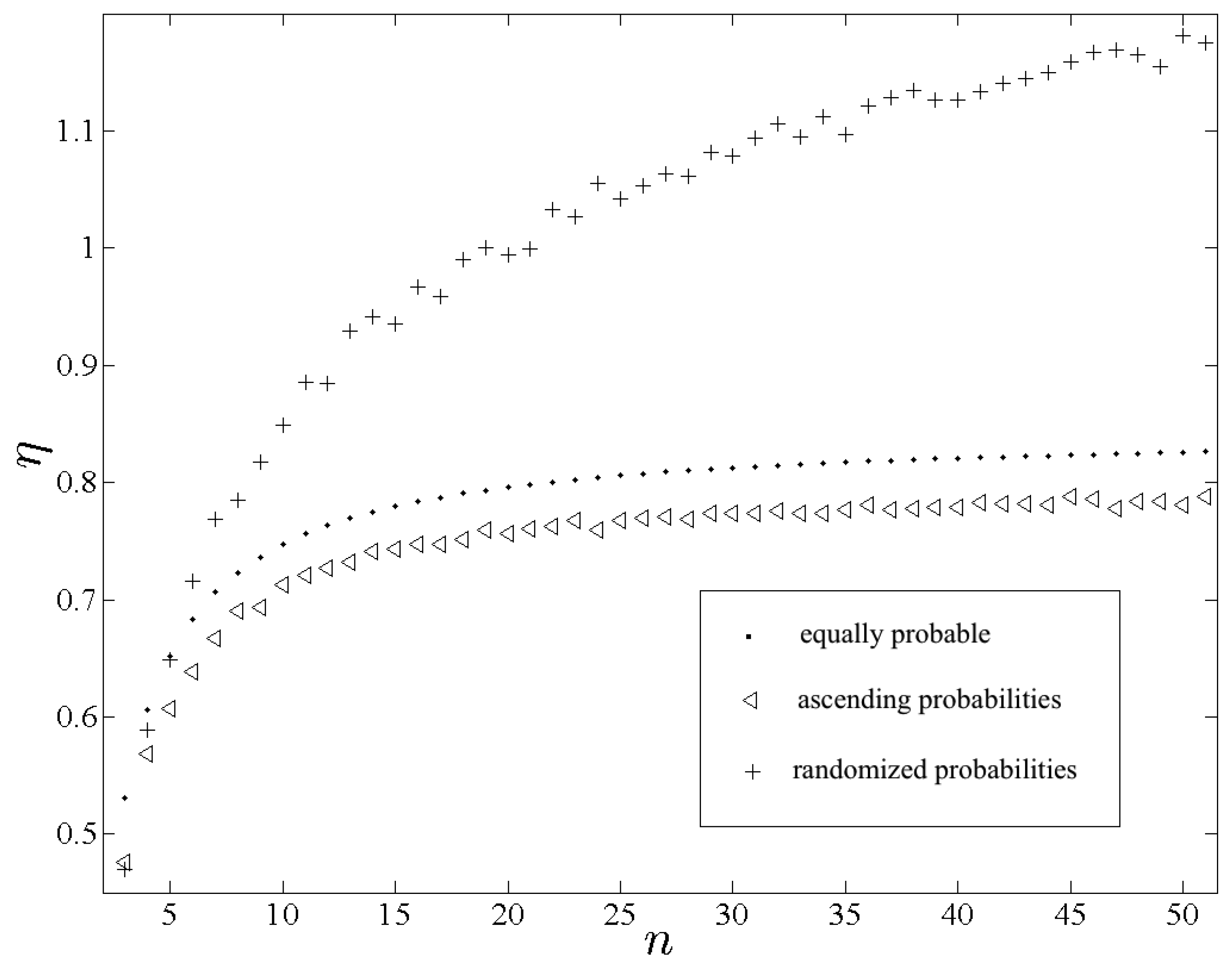
Let us begin by examining how η measures indeterminacy effected through different types of p. Figure 1 displays calculations of η(p_e, x_e), η(p_a, x_e) and η(p_r, x_e) plotted as functions of n. Recall that η(p_r, x_e) and η(p_a, x_e) should behave respectively as quantities of entropy attributed to the variables X_re and X_ae examined in Section 1. We find that η(p_r, x_e) is appreciably greater than η(p_a, x_e) for all but trivially small n, which is consistent with the expected result. Because the only difference between each p_a and p_r is the order of their respective terms, the differences between the associated quantities of entropy are entirely due to the contribution from Ξ.

Perhaps more importantly, and in opposition to the behavior of H alone, we find that $\eta ({\mathbf{p}}_r,{\mathbf{x}}_e)$ is also appreciably greater than $\eta ({\mathbf{p}}_e,{\mathbf{x}}_e)$ for all non-trivial n. Among generic discrete variables any non-uniformity in $\mathbf{p}$ is a benefit to predictability, hence $H\left({\mathbf{p}}_r\right)\le H\left({\mathbf{p}}_e\right)$. Among real-valued discrete variables, however, the predictive benefit of non-uniformities in $\mathbf{p}$ depends on the manner in which the probabilities are spatially assigned. In the case of $X_{re}$ the indeterminacy effected by the irregular spatial assignment of ${\mathbf{p}}_r$ evidently outweighs the intrinsic predictive benefit of ${\mathbf{p}}_r$, which implies that $X_{ee}$ behaves more deterministically than $X_{re}$. Though not necessarily expected a priori, that implication is not surprising.

Figure 1. Plots of $\eta ({\mathbf{p}}_e,{\mathbf{x}}_e)$, $\eta ({\mathbf{p}}_a,{\mathbf{x}}_e)$ and $\eta ({\mathbf{p}}_r,{\mathbf{x}}_e)$ using the respective symbols “•” , “◃” and “+”.

Figure 1. Plots of $\eta ({\mathbf{p}}_e,{\mathbf{x}}_e)$, $\eta ({\mathbf{p}}_a,{\mathbf{x}}_e)$ and $\eta ({\mathbf{p}}_r,{\mathbf{x}}_e)$ using the respective symbols “•” , “◃” and “+”.

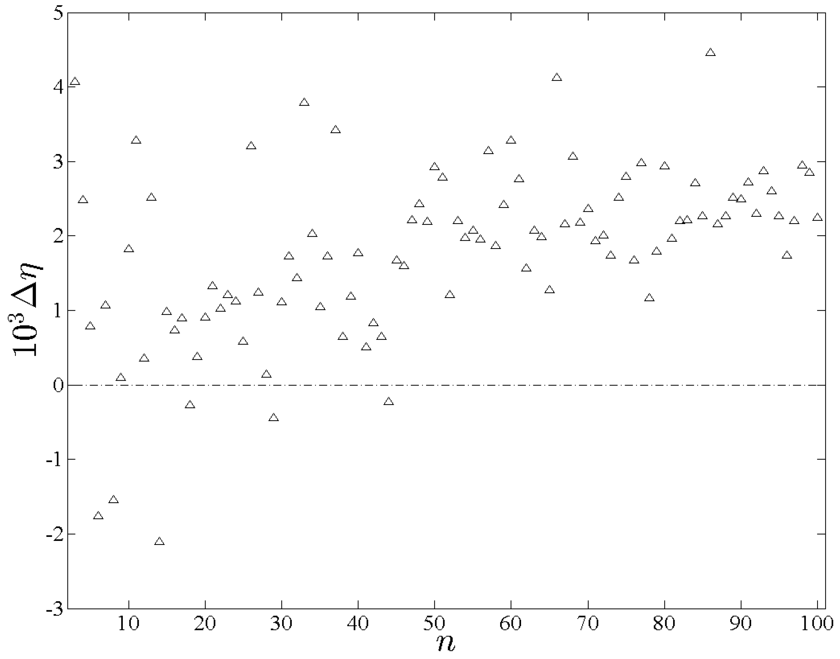
As a complement to the previous scenario it is instructive to compare the effects of the three types of probabilities when matched to spatially randomized outcomes. Figure 2 displays calculations of $\eta ({\mathbf{p}}_e,{\mathbf{x}}_r)$, $\eta ({\mathbf{p}}_a,{\mathbf{x}}_r)$ and $\eta ({\mathbf{p}}_r,{\mathbf{x}}_r)$ plotted as functions of n. Note that $\eta ({\mathbf{p}}_a,{\mathbf{x}}_r)$ and $\eta ({\mathbf{p}}_r,{\mathbf{x}}_r)$ nearly coincide for each n, and the symbols “⋄” and “*” are always superimposed in Figure 2. The entropy-difference $\eta ({\mathbf{p}}_r,{\mathbf{x}}_r)-\eta ({\mathbf{p}}_a,{\mathbf{x}}_r)$ is shown in Figure 3. In contrast to the previous scenario ${\mathbf{p}}_e$ consistently effects the largest entropy among the three, which is expected from Equation (52) given that $H\left({\mathbf{p}}_e\right)$ is maximal. Note that $\eta ({\mathbf{p}}_e,{\mathbf{x}}_r)$ would be even closer to $H\left({\mathbf{p}}_e\right)$ had the randomness of ${\mathbf{x}}_r$ not been restricted for the sake of computational feasibility. The similarity between $\eta ({\mathbf{p}}_r,{\mathbf{x}}_r)$ and $\eta ({\mathbf{p}}_a,{\mathbf{x}}_r)$ is also expected from Equation (52) given that $H\left({\mathbf{p}}_r\right)=H\left({\mathbf{p}}_a\right)$. Furthermore insofar as $\eta ({\mathbf{p}}_r,{\mathbf{x}}_r)$ and $\eta ({\mathbf{p}}_a,{\mathbf{x}}_r)$ differ the former should be typically greater for sufficiently large n, which is confirmed in Figure 3.

Let us next examine calculations demonstrating how η measures indeterminacy effected through x, which is perhaps the most significant attribute of η. The most basic comparison corresponds to the scenario involving $X_{ee}$ and $X_{er}$ in Section 1. It is immediately evident from Figure 1 and Figure 2 that $\eta ({\mathbf{p}}_e,{\mathbf{x}}_r)$ is considerably larger than $\eta ({\mathbf{p}}_e,{\mathbf{x}}_e)$ for all n, which is expected.

Figure 2. Plots of $\eta ({\mathbf{p}}_e,{\mathbf{x}}_r)$, $\eta ({\mathbf{p}}_a,{\mathbf{x}}_r)$ and $\eta ({\mathbf{p}}_r,{\mathbf{x}}_r)$, using the respective symbols “×”, “⋄” and “*”. The solid line follows a plot of $\log \left(n\right)$ for reference.

Figure 2. Plots of $\eta ({\mathbf{p}}_e,{\mathbf{x}}_r)$, $\eta ({\mathbf{p}}_a,{\mathbf{x}}_r)$ and $\eta ({\mathbf{p}}_r,{\mathbf{x}}_r)$, using the respective symbols “×”, “⋄” and “*”. The solid line follows a plot of $\log \left(n\right)$ for reference.

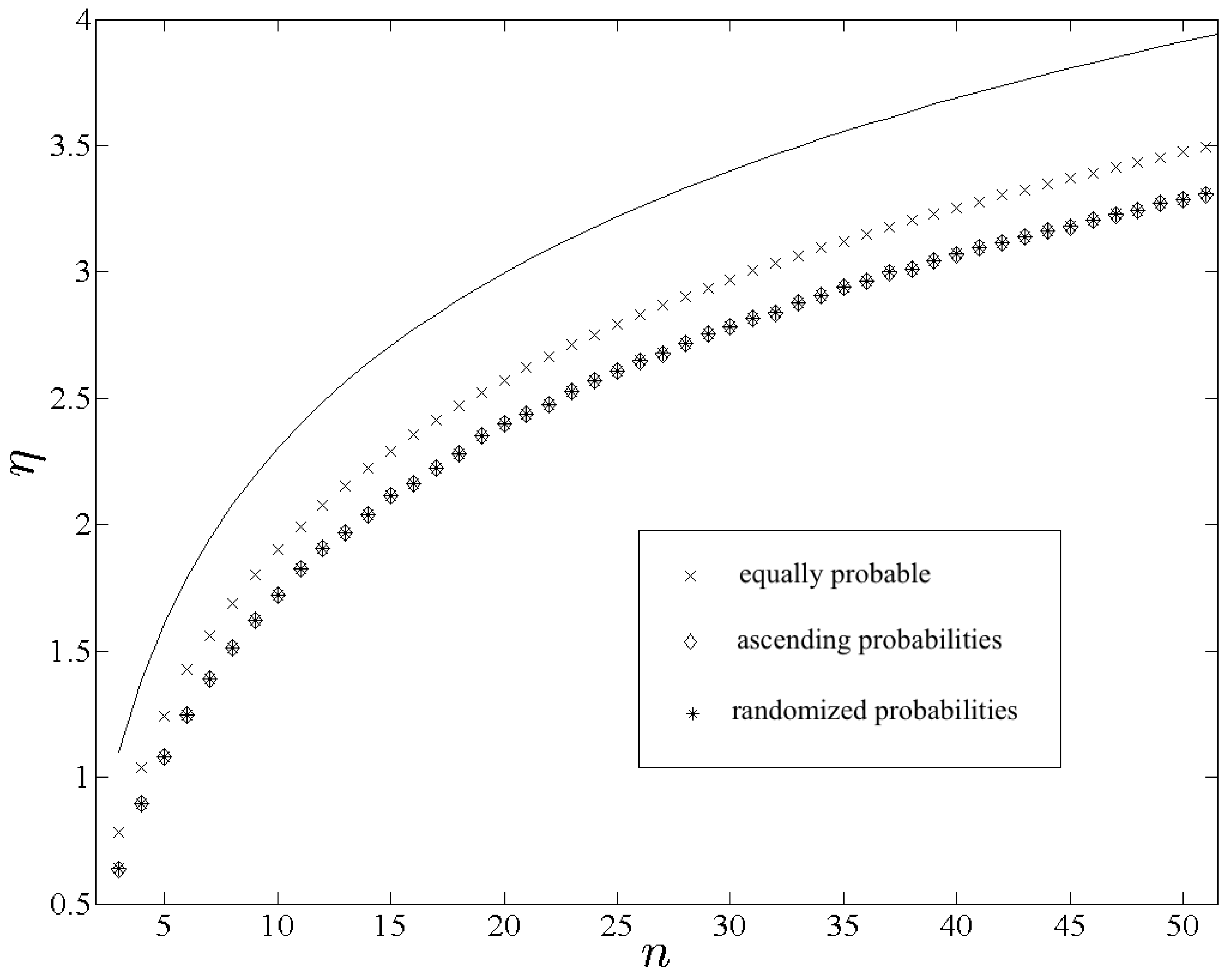
Figure 3. The entropy difference Δη plotted here is η(p_r,x_r) - η.(p_a, x_r).

Figure 3. The entropy difference Δη plotted here is η(p_r,x_r) - η.(p_a, x_r).

In order to test the sensitivity of η to more subtle differences in spatial structure the following additional sets of type $\mathbf{x}$ are defined. For a given n let x_p consist of the first n prime numbers. It follows from the Prime Number Theorem (PNT) that the local average gap in the vicinity of a given x_j ∈ x_p varies as log(j) for sufficiently large j. The term gap is used throughout in reference to a positive interval between consecutive terms in any given one-dimensional $\mathbf{x}$ and is defined such that the j-th gap is

$$g_j\equiv x_{j+1}-x_j$$

(56)

The global anisotropy associated with the PNT constitutes an intrinsic deterministic spatial characteristic. For a more pronounced anisotropy of the same kind, let ${\stackrel{,}{\text{x}}}_{\text{p}}=\{2,3\dots \}$ be defined for a given n such that its sequence of gaps consists of the first n − 1 prime gaps arranged in ascending order. As an example, for n = 6 we have ${\stackrel{,}{\text{x}}}_{\text{p}}=\{2,3,5,7,9,13\}$. Let ${\tilde{\text{x}}}_{\text{p}}=\{2,3\dots \}$ be defined for a given n such that its sequence of gaps consists of the first n − 1 prime gaps ordered randomly, with the exception that the first gap in ${\tilde{\text{x}}}_{\text{p}}$ is always 1. Finally let ${\breve{\text{x}}}_{\text{p}}=\{2,3\dots \}$ be defined such that its sequence of gaps is $g_1^{\prime },g_3^{\prime },g_2^{\prime },g_5^{\prime },g_4^{\prime },\dots$, where $g_j^{\prime }$ is the j-th prime gap. In other words, the sequence of gaps in ${\breve{\text{x}}}_{\text{p}}$ is constructed simply by alternating the order of $g_i^{\prime }$ and $g_{i+1}^{\prime }$ for all even i no greater than n − 2. Consequently every even-numbered element of ${\breve{\text{x}}}_{\text{p}}$ is guaranteed to be identical to the corresponding prime. As an example we have ${\breve{\text{x}}}_{\text{p}}=\{2,3,5,7,9,13,15,19\}$ for n = 8. Note that the average gap in the vicinity of some $x_j\in {\breve{\text{x}}}_{\text{p}}$ differs only negligibly from the corresponding average gap in the primes, and ${\breve{\text{x}}}_{\text{p}}$ therefore exhibits the same global anisotropy inherent to x_p.

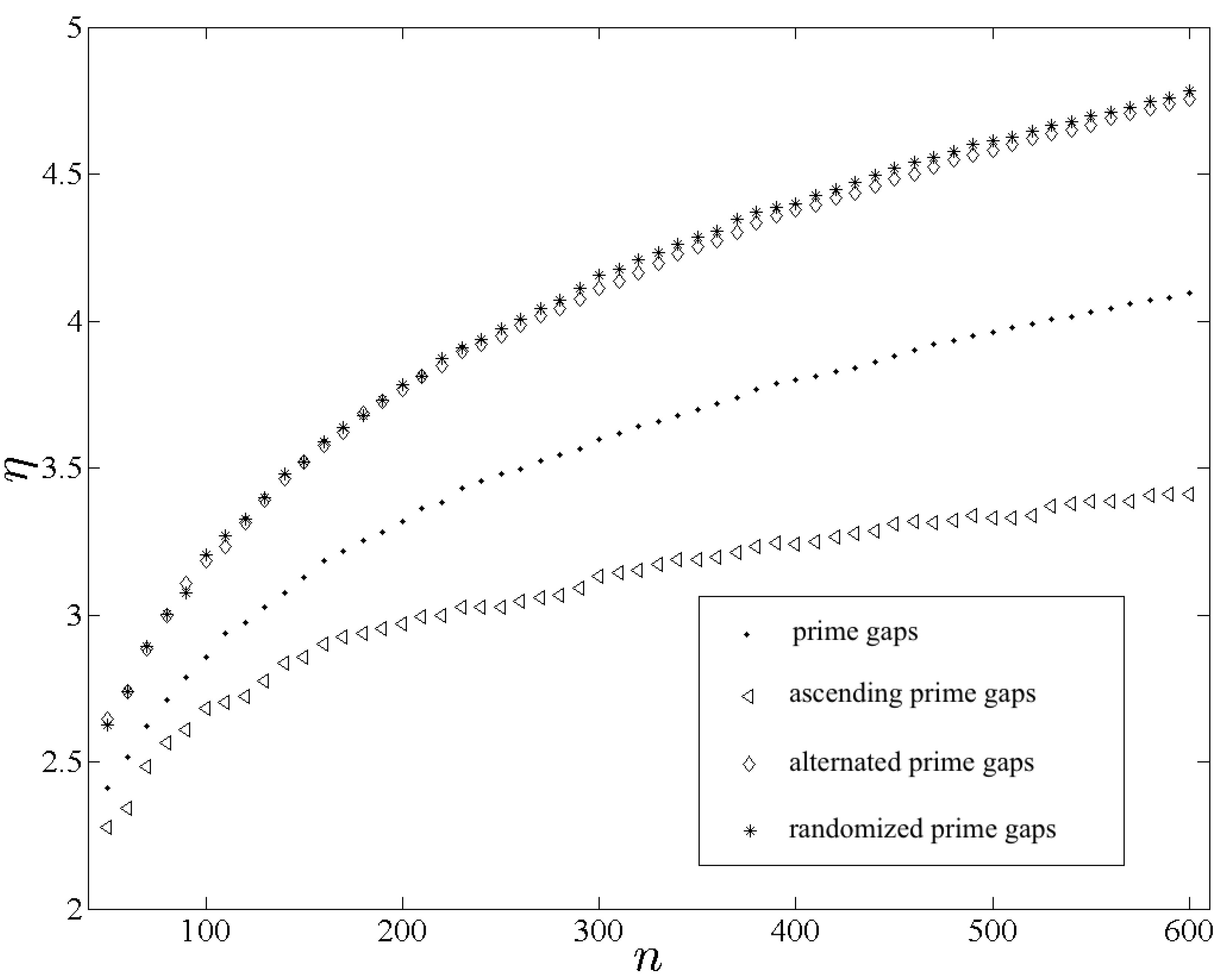
Consider four variables with $n\gg 1$ allowed outcomes ${\mathbf{x}}_p$, ${\acute{\mathbf{x}}}_p$, ${\tilde{\mathbf{x}}}_p$ and ${\breve{\mathbf{x}}}_p$, respectively, all of which are equally probable. As ${\tilde{\mathbf{x}}}_p$ is the least deterministically configured among the four, $\eta ({\mathbf{p}}_e,{\tilde{\mathbf{x}}}_p)$ should be largest. Furthermore, given that the sequence of gaps in ${\acute{\mathbf{x}}}_p$ ascends uniformly, the deterministic nature of the associated anisotropy is significantly greater than in ${\mathbf{x}}_p$ and ${\breve{\mathbf{x}}}_p$. We therefore expect $\eta ({\mathbf{p}}_e,{\acute{\mathbf{x}}}_p)$ to be the smallest entropy among the four. Figure 4 shows $\eta ({\mathbf{p}}_e,{\mathbf{x}}_p)$, $\eta ({\mathbf{p}}_e,{\acute{\mathbf{x}}}_p)$, $\eta ({\mathbf{p}}_e,{\tilde{\mathbf{x}}}_p)$ and $\eta ({\mathbf{p}}_e,{\breve{\mathbf{x}}}_p)$ plotted as functions of n. Although $\eta ({\mathbf{p}}_e,{\tilde{\mathbf{x}}}_p)$ and $\eta ({\mathbf{p}}_e,{\breve{\mathbf{x}}}_p)$ differ only negligibly for n smaller than approximately 200, for all larger n the entropy due to ${\tilde{\mathbf{x}}}_p$ is the greatest among the four. The small but non-negligible difference between $\eta ({\mathbf{p}}_e,{\tilde{\mathbf{x}}}_p)$ and $\eta ({\mathbf{p}}_e,{\breve{\mathbf{x}}}_p)$ for large n is attributed to the global anisotropy in ${\breve{\mathbf{x}}}_p$. The entropy due to ${\acute{\mathbf{x}}}_p$ is the smallest among the four. The behavior of η in these calculations is therefore consistent with the stated expectations.

The dramatic difference between $\eta ({\mathbf{p}}_e,{\mathbf{x}}_p)$ and $\eta ({\mathbf{p}}_e,{\breve{\mathbf{x}}}_p)$ is noteworthy and unexpected. The smaller entropy due to ${\mathbf{x}}_p$ implies a greater degree of intrinsic determinacy in the arrangement of ${\mathbf{x}}_p$ along the real axis. Note that the implied deterministic structure could not be associated with the PNT. A detailed analysis of this finding is beyond the present scope and has become the subject of a separate investigation [12]. For the present purposes it is sufficient to mention, as the reader may verify readily, that the number of positive intervals of a given size d among the first $n\gg 1$ primes is strongly correlated to the largest primordial factor of d [12]. That regularity could represent the deterministic property intimated by ${\mathbf{p}}_e,{\mathbf{x}}_p)$.

Figure 4. Plots of $\eta ({\mathbf{p}}_e,{\mathbf{x}}_p)$, $\eta ({\mathbf{p}}_e,{\acute{\mathbf{x}}}_p)$, $\eta ({\mathbf{p}}_e,{\breve{\mathbf{x}}}_p)$ and $\eta ({\mathbf{p}}_e,{\tilde{\mathbf{x}}}_p)$, shown with “•”, “◃”, “⋄” and “*”, respectively, measuring intrinsic structure in the primes ${\mathbf{x}}_p$ and in three variants constructed by changing the order of the first $n-2$ even prime gaps.

Figure 4. Plots of $\eta ({\mathbf{p}}_e,{\mathbf{x}}_p)$, $\eta ({\mathbf{p}}_e,{\acute{\mathbf{x}}}_p)$, $\eta ({\mathbf{p}}_e,{\breve{\mathbf{x}}}_p)$ and $\eta ({\mathbf{p}}_e,{\tilde{\mathbf{x}}}_p)$, shown with “•”, “◃”, “⋄” and “*”, respectively, measuring intrinsic structure in the primes ${\mathbf{x}}_p$ and in three variants constructed by changing the order of the first $n-2$ even prime gaps.

5. Summary and Conclusions

For finite ν the entropy attributed to the variable ${\mathcal{X}}_{\mathit{X}}$ governed by ${\rho }_{\mathit{X}}(\nu ,x)$ is simply $\mathcal{H}\left({\rho }_{\mathit{X}}\right)$. In the limit as $\nu \to \infty$, however, ${\mathcal{X}}_{\mathit{X}}$ becomes a discrete variable X whose behavior is insensitive to the function ${\rho }_0$ from which ${\rho }_{\mathit{X}}$ is constructed. The entropy attributed asymptotically to X is therefore $\mathcal{H}\left({\rho }_{\mathit{X}}\right)-\mathcal{H}\left({\rho }_0\right)$, which recovers the discrete Shannon entropy. Similarly when ν is finite a quantity of entropy $S\left({\psi }_{\mathit{X}}\right)$ is attributed to the conjugated pair ${\mathcal{X}}_{\mathit{X}}$ and ${\mathcal{K}}_{\mathit{X}}$. The nature of the pair, however, is asymptotically insensitive to ${\varphi }_0$. The entropy attributed to the pair in the limit as ν diverges is therefore $S\left({\psi }_{\mathit{X}}\right)-S\left({\varphi }_0\right)$, whose asymptotic form $H+\Xi$ is defined as η. Furthermore because the conjugate is asymptotically eliminated η must be attributed to X alone.

As H is a function only of $\mathbf{p}$, the existence of some $\mathbf{x}$-dependent contribution to the entropy of a discrete real variable is expected independently of the introduction of Ξ. Whereas the form of H uniquely exhibits the properties required for a self-consistent measure of indeterminacy effected by $\mathbf{p}$ [1], the complete set of requirements for a measure of indeterminacy effected by $\mathbf{x}$ and $\mathbf{p}$ is not readily ascertained a priori. Among those required properties are certainly translational invariance, scale-invariance, rotational invariance, non-negativity and being bound from above by H, all of which were proven for η Section 3. Furthermore the calculations presented in Section 4 demonstrate that η behaves in the expected manner over a broad range of different configurations of $\mathbf{x}$ and $\mathbf{p}$.

The somewhat counterintuitive role of Ξ is a natural consequence of the relationship between a given wave-mechanical probability density and the corresponding spectral density. More broadly interpreted, the wave-mechanical origin of η may be understood as a natural consequence of a fundamental unity between information theory and quantum theory. Such an interpretation is well-motivated given the profound connections already known. For instance, the bounds on S lead to an uncertainty relation that is stronger than the most general form of the Heisenberg Uncertainty Principle [2]. Even more striking, the basic precepts of quantum theory have been derived from informatic principles [13].It is important to specify, however, that the validity of η is contingent upon no quantum-mechanical premise.

The distinctive feature of η is its dependence on x, which is necessary for a complete measure of indeterminacy in discrete real variables. Because of the generality of its form, η can be readily manipulated to probe intrinsic organization in sequences of real numbers. Section 4 presented calculations demonstrating the novel capability ofη in such applications. Future investigations will explore additional applications of η.

References

- Shannon, C.E. A mathematical theory of communication. Bell. Syst. Tech. J. 1948, 27, 379. [Google Scholar] [CrossRef]
- Bialynicki-Birula, I.; Mycielski, J. Uncertainty relations for information entropy in wave mechanics. Commun. Math. Phys. 1975, 44, 129–132. [Google Scholar] [CrossRef]
- Gadre, S.R.; Bendale, R.D. Rigorous relationships among quantum-mechanical kinetic energy and atomic information entropies: Upper and lower bounds. Phys. Rev. A 1987, 36, 1932–1935. [Google Scholar] [CrossRef] [PubMed]
- Lalazissis, G.A.; Massen, S.E.; Panos, C.P.; Dimitrova, S.S. Information entropy as a measure of the quality of a nuclear density distribution. Int. J. Mod. Phys. E 1998, 7, 485–494. [Google Scholar] [CrossRef]
- Guevara, N.L.; Sagar, R.P.; Esquivel, R.O. Shannon-information entropy sum as a correlation measure in atomic systems. Phys. Rev. A 2003, 67, 012507. [Google Scholar] [CrossRef]
- Massen, S.E. Application of information entropy to nuclei. Phys. Rev. C 2003, 67, 014314. [Google Scholar] [CrossRef]
- Shi, Q.; Kais, S. Discontinuity of Shannon information entropy for two-electron atoms. J. Chem. Phys. 2004, 309, 127–131. [Google Scholar] [CrossRef]
- Bialynicki-Birula, I.; Rudnicki, L. Entropic uncertainty relations in quantum physics. In Statistical Complexity; Sen, K.D., Ed.; Springer: Berlin, Heidelberg, Germany, 2007; pp. 1–34. [Google Scholar]
- Ghosh, S.K.; Berkowitz, M.; Parr, R.G. Transcription of ground-state density-functional theory into a local thermodynamics. Proc. Natl. Acad. Sci. USA 1984, 81, 8028. [Google Scholar] [CrossRef] [PubMed]
- Kullback, S.; Leibler, R.A. On information and sufficiency. Annals Math. Stat. 1951, 22, 79–86. [Google Scholar] [CrossRef]
- Feynman, R.P. Theory of Fundamental Processes; W. A. Benjamin, Inc.: New York, NY, USA, 1962; pp. 1–6. [Google Scholar]
- Cartwright, C.; Funkhouser, S.; Sengupta, D.; Williams, B. Periodicity in the intervals between primes. Am. J. Comput. Math. 2012. submitted for publication. [Google Scholar]
- Chiribella, G.; D’Ariano, G.M.; Perinotti, P. Informational derivation of quantum theory. Phys. Rev. A 2011, 84, 012311. [Google Scholar] [CrossRef]
© 2012 by the author; licensee MDPI, Basel, Switzerland. This article is an open access article distributed under the terms and conditions of the Creative Commons Attribution license (http://creativecommons.org/licenses/by/3.0/).
Share and Cite
MDPI and ACS Style
Funkhouser, S. The Entropy of a Discrete Real Variable. Entropy 2012, 14, 1522-1538. https://doi.org/10.3390/e14081522
AMA Style
Funkhouser S. The Entropy of a Discrete Real Variable. Entropy. 2012; 14(8):1522-1538. https://doi.org/10.3390/e14081522
Chicago/Turabian StyleFunkhouser, Scott. 2012. "The Entropy of a Discrete Real Variable" Entropy 14, no. 8: 1522-1538. https://doi.org/10.3390/e14081522