Bearing Fault Diagnosis Based on Multiscale Permutation Entropy and Support Vector Machine

Abstract

Bearing fault diagnosis has attracted significant attention over the past few decades. It consists of two major parts: vibration signal feature extraction and condition classification for the extracted features. In this paper, multiscale permutation entropy (MPE) was introduced for feature extraction from faulty bearing vibration signals. After extracting feature vectors by MPE, the support vector machine (SVM) was applied to automate the fault diagnosis procedure. Simulation results demonstrated that the proposed method is a very powerful algorithm for bearing fault diagnosis and has much better performance than the methods based on single scale permutation entropy (PE) and multiscale entropy (MSE).

1. Introduction

Bearings are the most frequently used component in a rotary machine. Bearing failures could lead to unpredictable productivity losses for production facilities. Therefore, bearing fault diagnosis has attracted significant attention from the research and engineering communities over the past decades. Generally, a bearing fault diagnosis process can be decomposed into three steps: data acquisition, feature extraction, and fault condition classification.

Vibration-based signal analysis in the time-frequency domain has been a major technique for bearing fault diagnosis. Several statistical parameters in the time domain and the frequency domain, such as the root mean square, kurtosis, and skewness, have been shown to be capable of fault detection [1,2]. In [1], nine features in the time domain and seven features in the frequency domain were used for bearing fault detection. We call this method the time domain and frequency domain statistical formulas (TDFDSFs) method throughout this paper.

Time-frequency analysis methods, such as the short-time Fourier transform [3], the Wigner Ville distribution [4], and the wavelet transform [5], have been widely used to detect bearing faults since they can provide abundant information about machine faults. However, these time-frequency based methods often require a lot of computation time, as they involve a lot of Fourier transforms or convolution operations. Moreover, due to the factors of clearance and nonlinear stiffness of bearings, the vibration signals are often characterized by nonlinearity. Therefore, these commonly used time-frequency analysis techniques may exhibit limitations because of their linearity assumption.

In order to overcome this problem, several nonlinear parameter estimation techniques were applied to extract defect-related features hidden in the measured signals. In [6], Hong and Liang combined the Lempel-Ziv complexity with the continuous wavelet transform and found that the new method was more effective in bearing fault diagnosis. Then, the methods based on approximate entropy (ApEn) [7] and multiscale entropy (MSE) [8] were used for bearing fault diagnosis. Both ApEn and MSE can be used for measuring the regularity of a time series. Although these entropy-based methods are simple and require much less computation time, they have very good performance in bearing fault diagnosis.

In [9], a new entropy based method named permutation entropy (PE) was exploited to assess the status of a rotary machine. The PE was introduced by Bandit [10]. It estimates the complexity of time series through the comparison of neighboring values. The PE has been widely used in a number of applications, such as electroencephalography (EEG) signal analysis [11,12], stock market analysis [13], tool breakage detection in end milling [14], and chatter detection in turning processes [15]. Time series derived from physiological and mechanical systems are usually complicated and consist of multiple temporal scale structures. Based on a single scale algorithm, the PE based method has limited performance in analyzing these complicated data. To overcome this shortcoming, based on the concept of multiscale [16], Aziz proposed a new method termed mutliscale permutation entropy (MPE) to calculate entropy over multiple scales [17]. In addition, Li employed the MPE method to track the effect of anesthetic drug sevoflurane on the brain and showed that the MPE index outperforms the single scale PE index [18].

In this paper, we introduce MPE as a feature extractor of the bearing fault diagnosis system. After extracting feature vectors by MPE, the multi-class support vector machine (SVM) [19] is used as a classifier. The SVM is probably the most popular and powerful machine learning algorithm because of its well established theoretical background and intuitive geometrical interpretation. Nowadays, the SVM is widely applied and has even served as the baseline in computer vision, pattern recognition, information retrieval, and data mining, etc. In our simulations, the vibration signal datasets of bearing from Case Western Reserve University (CWRU) [20] are utilized. Experimental results demonstrate that the proposed MPE-based algorithm provides a significantly higher accuracy of prediction than the traditional feature extraction methods.

The remainder of this paper is organized as follows: Section 2 provides a review of permutation entropy. In Section 3, the proposed algorithm based on multiscale permutation entropy is introduced. In Section 4, several examples are presented to demonstrate the effectiveness of the proposed MPE algorithm. A conclusion is given in Section 5.

2. Permutation Entropy

Given a time series {x(k), k = 1, 2, …, N}, the m-dimensional delay embedding vector at time i is defined as:

$$x_i^m=\left[x(i),x(i+\tau ),\cdots ,x(i+(m-1))\tau \right]$$

(1)

where m is the embedded dimension and τ is time delay. We say that $x_i^m$ has a permutation ${\pi }_{r_o{r}_1\mathrm{...}{r}_{m-1}}$ if it satisfies:

$$x(t+r_o\tau )\le x(t+r_1\tau )\le \cdots \le x(t+r_{m-1}\tau )$$

(2)

where 0 ≤ r_i ≤ m − 1 and r_i ≠ r_j.

There are m! possible permutations of for an m-tuple vector. For each permutation π, we determine the relative frequency by:

$$p(\pi )=\frac{Number\left\{t|t\le T-(m-1)\tau ,x_t^m\text{ has type }\pi \right\}}{N-(m-1)\tau }$$

(3)

The PE of m dimension is then defined as:

$$H_{\text{PE}}(m)=-{\displaystyle \sum p(\pi )\ln (p(\pi ))}$$

(4)

The maximum value of H_PE(m) is log(m!) when all possible permutations appear with the same probability. Therefore, the normalized permutation entropy (NPE) can be obtained as:

$$H_{\text{NPE}}(m)=\raisebox{1ex}{$H_{\text{PE}}(m)$}\!\left/ \!\raisebox{-1ex}{$\ln (m!)$}\right.$$

(5)

For any time series, 0 ≤ H_NPE(m) ≤ 1 is satisfied.

In the remainder of this section, we explain the PE algorithm by using an example of the time series in Equation (6):

$$x=\left(4,7,9,10,6,11,3\right)$$

(6)

We set the parameter of time delay τ to be 1. When the embedded dimension m is 3, five embedding vectors can be obtained as:

$$\left[\begin{array}{c}{x}_1^3\\ x_2^3\\ x_3^3\\ x_4^3\\ x_5^3\end{array}\right]=\left[\begin{array}{ccc}4& 7& 9\\ 7& 9& 10\\ 9& 10& 6\\ 10& 6& 11\\ 6& 11& 3\end{array}\right]$$

(7)

There are six (3!) possible permutations of dimension 3, which are denoted by π₀₁₂, π₀₂₁, π₁₀₂, π₁₂₀, π₂₀₁, and π₂₁₀, respectively. The embedding vectors $x_1^3$ and $x_2^3$ have the permutation type π₀₁₂, the vector $x_4^3$ has the permutation type π₁₀₂, while both $x_3^3$ and $x_5^3$ correspond to π₂₀₁. Therefore, the probability of each permutation is given by:

$$\begin{array}{l}p({\pi }_{012})=\frac{2}{5},p({\pi }_{021})=0,p({\pi }_{102})=\frac{1}{5},\\ p({\pi }_{120})=0,p({\pi }_{201})=\frac{2}{5},p({\pi }_{210})=0.\end{array}$$

(8)

The PE and the NPE of dimension 3 are then calculated by:

$$H_{\text{PE}}(m)=-\raisebox{1ex}{$2$}\!\left/ \!\raisebox{-1ex}{$5$}\right.\ln (\raisebox{1ex}{$2$}\!\left/ \!\raisebox{-1ex}{$5$}\right.)-\raisebox{1ex}{$1$}\!\left/ \!\raisebox{-1ex}{$5$}\right.\ln (\raisebox{1ex}{$1$}\!\left/ \!\raisebox{-1ex}{$5$}\right.)-\raisebox{1ex}{$2$}\!\left/ \!\raisebox{-1ex}{$5$}\right.\ln (\raisebox{1ex}{$2$}\!\left/ \!\raisebox{-1ex}{$5$}\right.)\approx 1.0549$$

(9)

$$H_{\text{NPE}}(m)=\frac{1.0549}{\ln (3!)}=0.5888$$

(10)

The value of PE depends on the selection of the embedding dimension m and delay τ. If m is too small, the scheme will not work since there are too few distinct states. However, it is often inappropriate to choose m as a large value for detecting the dynamic change of a time series [17]. Moreover, Cao [21] indicated that the delay τ is related to the signal for analysis and its sampling rate.

3. Proposed Bearing Fault Diagnosis System Based on Multiscale Permutation Entropy and Support Vector Machine

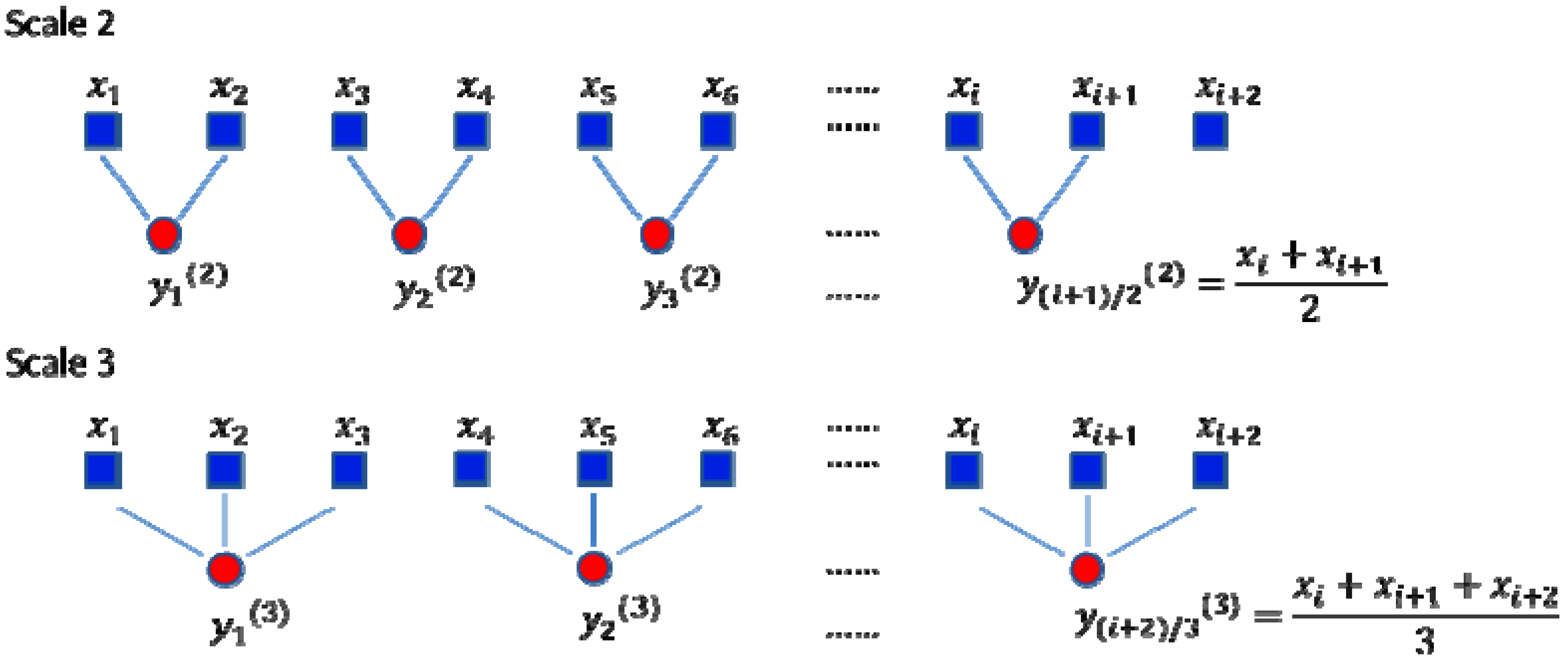
The concept of multiscale analysis was originally proposed by Costa [16], who indicated that the single scale entropy algorithm yielded contradictory results when applied to real-world datasets obtained in health and disease states. In regard to this, Costa proposed a coarse-grained procedure to obtain multiple scale time series from the original time series. Then, the entropy at each scale is calculated to analyze the physiological signal. Given a time series x = {x₁, x₂, …, x_N}, one can construct a consecutive coarse-grained time series y^(s) corresponding to the time scale s. First, the original time series is divided into non-overlapping windows of length s. Second, the data points inside each window are averaged by Equation (11). The schematic illustration of the coarse-grained procedure is shown as in Figure 1:

$$y_j^{(s)}=\frac{1}{s}{\displaystyle \sum _{i=(j-1)s+1}^{js}{x}_i},1\le j\le \frac{N}{s}$$

(11)

Figure 1. Schematic illustration of the coarse-grained procedure modified from [16].

Figure 1. Schematic illustration of the coarse-grained procedure modified from [16].

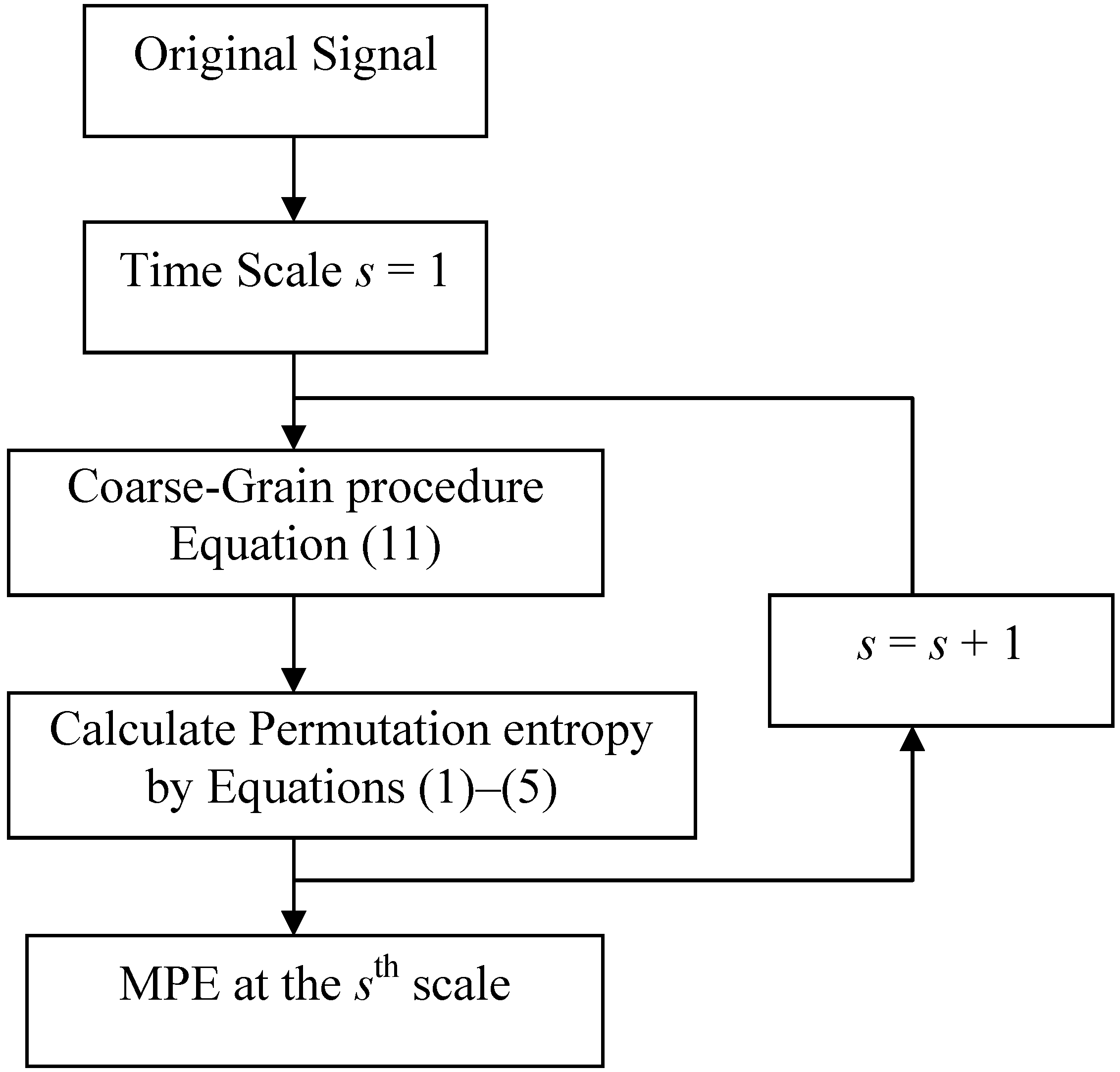
Based on the concepts of multiscale and PE, Aziz proposed a new method termed mutliscale permutation entropy (MPE). In MPE analysis, the entropy of the coarse-grained time series at each scale is calculated by the NPE algorithm defined in Equations (3)–(5). Li employed MPE analysis to track the effect of anesthetic drug sevoflurane on the brain and showed that the MPE index outperforms the single scale PE index [18]. In this paper, motivated by the previous efforts, we investigate the utility of MPE for detecting a variety of bearing faults in rotary machines. The flowchart of the multiscale permutation entropy algorithm is as seen in Figure 2.

Figure 2. Flowchart of the multiscale permutation entropy algorithm.

Figure 2. Flowchart of the multiscale permutation entropy algorithm.

In addition to multiscale permutation entropy, our proposed method also adopts the SVM technique. The SVM was originally a deterministic algorithm for finding the linear separating hyperplane of a binary labeled dataset. Compared to the perceptron learning algorithm (PLA), which eventually finds a random separating hyperplane in a linear-separable dataset, the SVM generates a unique hyperplane in a given dataset. This hyperplane provided by the SVM not only has an intuitive geometrical interpretation, but also been proved theoretically to balance the in-sample error (E_in) and the generalization error.

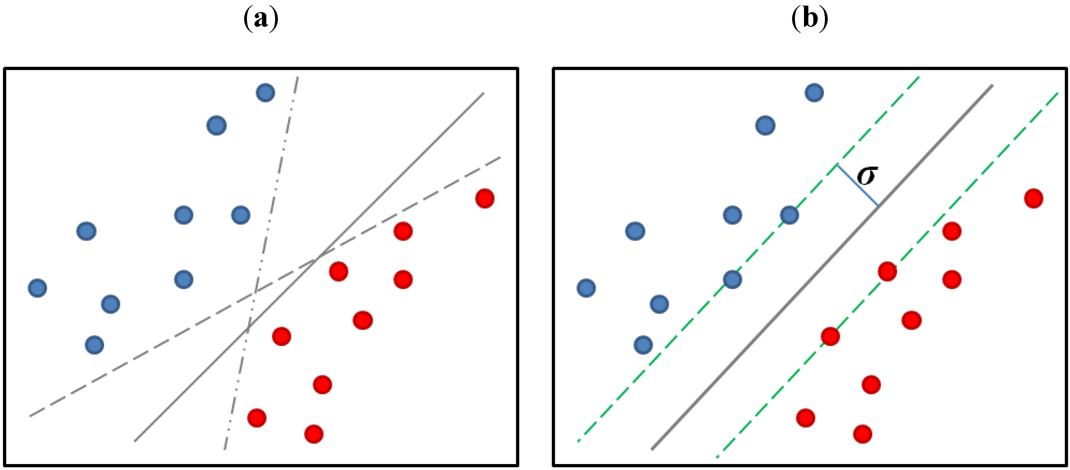
Given a binary labeled dataset as shown in Figure 3, we found that there are many hyperplanes that can be used to separate red circles (positive: 1) from blue circles (negative: −1), such as the three gray lines plotted in Figure 3a. These gray lines may come from the PLA, the Adaline algorithm, the least square regression algorithm, or the logistic regression algorithm, where the last three ones determine their separating hyperplanes based on the corresponding objective functions but without a direct geometrical interpretation. By contrast, the SVM was originated from a geometrical view as shown in Figure 3b. It seeks a separating hyperplane which keeps its distance from the positive and negative samples as far as possible without training error. In other words, the SVM desires a separating hyperplane that can maximize the margin σ between the positive and the negative samples. It can effectively tolerate the error of the unseen samples and was claimed to have good generalization ability. The objective function of the SVM is then modeled as a constraint optimization problem. In our algorithm, the SVM classifier is implemented by the LIBSVM software [20].

Figure 3. Different separating hyperplanes resulted from different algorithms: (a) the hyperplanes (three gray lines) resulted from general linear classification algorithms; (b) the hyperplane (gray line) resulted from the linear SVM algorithm where the margin σ is the distance between the hyperplane and the nearest sample.

Figure 3. Different separating hyperplanes resulted from different algorithms: (a) the hyperplanes (three gray lines) resulted from general linear classification algorithms; (b) the hyperplane (gray line) resulted from the linear SVM algorithm where the margin σ is the distance between the hyperplane and the nearest sample.

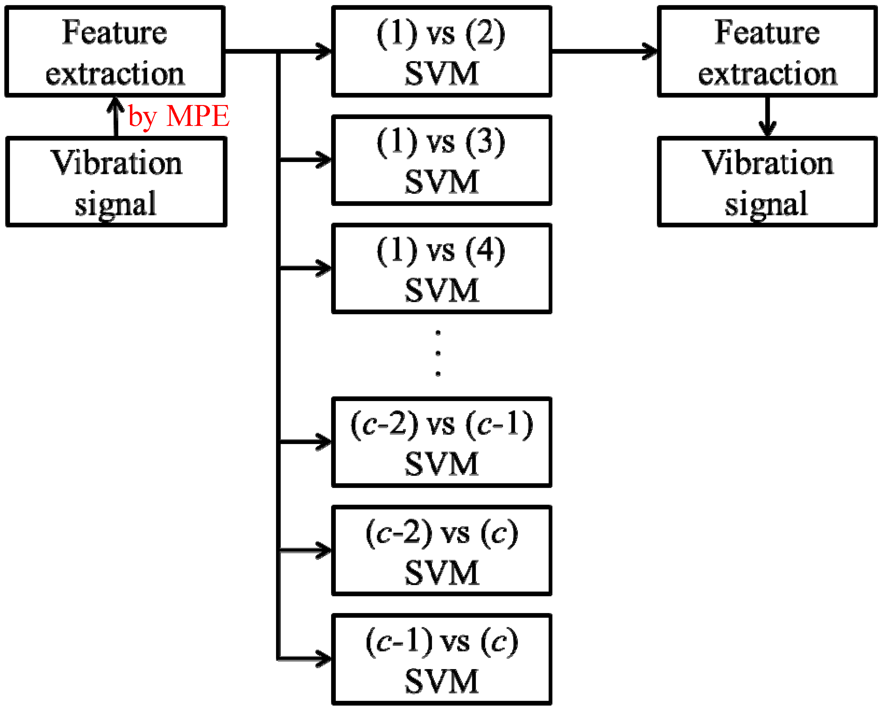
The overall flowchart of our proposed framework is shown in Figure 4. As recommended in [20], each feature is rescaled to the range of 0 to 1. The one-versus-one (OVO) SVM is chosen to classify different bearing faults. Assume that there are totally c classes. The OVO SVM builds a binary classifier for each pair of classes, which means that, in sum, c(c − 1)/2 binary classifiers are built. When given an input sample x, each classifier predicts a possible class label. The final predicted label is the one with the most votes among all c(c − 1)/2 classifiers.

Figure 4. The flowchart of our framework with the one-versus-one SVM of c classes.

Figure 4. The flowchart of our framework with the one-versus-one SVM of c classes.

4. Simulation Results

4.1. Experimental Data

In order to validate the capability of the MPE algorithm, experimental analyses on bearing faults were conducted. All the bearing data we used were obtained from the CWRU Bearing Data Center [4]. The time-domain vibration signals of bearing were collected from the normal case, the ball fault case, the inner race fault case, and the case of the outer race fault at the 6 o’clock position. The shaft rotating speeds of the motor are 1730, 1750, 1772, and 1797 rpm, and the sampling frequency is 48 kHz. For all fault conditions, the defect size of point fault is 14 mil in diameter.

In these experiments, the vibration signals collected from different fault conditions are divided into several non-overlapping 2048-point width windows. The window number of each fault condition at a specific rotating speed is shown in Table 1. Then, in Table 2, Table 3, Table 4, Table 5, Table 6, Table 7, Table 8 and Table 9, the method of time domain and the frequency domain statistical formulas (TDFDSFs) [1], the MSE method [8,16], the PE method [10,16], and the proposed MPE method were used to extract the features and their performances compared.

Table 1. The window number of each fault condition.

Actual Class	The motor shaft rotation speeds
	1730 rpm	1750 rpm	1772 rpm	1797 rpm
Normal	237	236	236	119
Ball fault	237	237	237	121
Inner race	236	238	186	31
outer race	238	237	236	119

Table 1. The window number of each fault condition.

Actual Class	The motor shaft rotation speeds
	1730 rpm	1750 rpm	1772 rpm	1797 rpm
Normal	237	236	236	119
Ball fault	237	237	237	121
Inner race	236	238	186	31
outer race	238	237	236	119

To demonstrate the effect of the number of training samples, the experiments were designed by different training set sizes (10%, 20%, 30%, 40%, and 50% of total samples), and the remaining samples are used for prediction. The average accuracy of prediction for each experiment was quantified over 200 tests.

4.2. Results

The average accuracies of prediction for different feature extraction methods are presented in Table 2, Table 3, Table 4 and Table 5. In the experiments, 16 TDFDSF features, 16 MSE features, a single PE feature and 16 MPE features were used to train the corresponding SVM model. The parameter r of MSE was set to 0.15σ where σ represents the standard deviation of original signals. The embedded dimension m and the time delay τ of MPE were set to 5 and 1, respectively. The parameters C and γ, of the SVM were 100 and the reciprocal of the feature number, respectively. As presented in Table 2, Table 3, Table 4 and Table 5, in the cases where the percentages of training samples are 10%, 20%, 30%, 40%, and 50%, the accuracies of the MPE based fault diagnosis system are all superior to those of the TDFDSF, the MSE, and the single scale PE based fault diagnosis systems. As shown by the experimental results, the single scale PE (i.e., MPE at scale 1) is not good enough to classify different bearing faults. However, a fault diagnosis system with the accuracy of prediction up to 99% will be obtained if MPE features are used. Another advantage of the MPE is that it is more robust on the variation of the training size. The computational cost for the SVM training procedure can be greatly reduced since a large number of training samples are unnecessary.

Table 2. The average accuracies at 1730 rpm.

Actual Class	Amount of training windows
	10%	20%	30%	40%	50%
TDFDSFs	90.34%	91.56%	92.03%	92.55%	92.89%
PE	73.19%	74.02%	74.25%	74.43%	74.59%
MSE	98.26%	98.79%	99.08%	99.14%	99.30%
MPE	99.15%	99.31%	99.43%	99.55%	99.55%

Table 2. The average accuracies at 1730 rpm.

Actual Class	Amount of training windows
	10%	20%	30%	40%	50%
TDFDSFs	90.34%	91.56%	92.03%	92.55%	92.89%
PE	73.19%	74.02%	74.25%	74.43%	74.59%
MSE	98.26%	98.79%	99.08%	99.14%	99.30%
MPE	99.15%	99.31%	99.43%	99.55%	99.55%

Table 3. The average accuracies at 1750 rpm.

Actual Class	Amount of training windows
	10%	20%	30%	40%	50%
TDFDSFs	81.26%	84.55%	85.65%	86.40%	87.09%
PE	75.60%	75.67%	75.78%	75.43%	75.35%
MSE	96.53%	97.53%	97.86%	98.12%	98.23%
MPE	99.99%	99.99%	99.99%	99.99%	99.99%

Table 3. The average accuracies at 1750 rpm.

Actual Class	Amount of training windows
	10%	20%	30%	40%	50%
TDFDSFs	81.26%	84.55%	85.65%	86.40%	87.09%
PE	75.60%	75.67%	75.78%	75.43%	75.35%
MSE	96.53%	97.53%	97.86%	98.12%	98.23%
MPE	99.99%	99.99%	99.99%	99.99%	99.99%

Table 4. The average accuracies at 1772 rpm.

Actual Class	Amount of training windows
	10%	20%	30%	40%	50%
TDFDSFs	87.77%	90.06%	91.47%	92.27%	92.96%
PE	75.09%	75.09%	75.75%	76.30%	76.92%
MSE	94.02%	9494%	95.14%	95.30%	95.63%
MPE	99.43%	99.63%	99.72%	99.78%	99.82%

Table 4. The average accuracies at 1772 rpm.

Actual Class	Amount of training windows
	10%	20%	30%	40%	50%
TDFDSFs	87.77%	90.06%	91.47%	92.27%	92.96%
PE	75.09%	75.09%	75.75%	76.30%	76.92%
MSE	94.02%	9494%	95.14%	95.30%	95.63%
MPE	99.43%	99.63%	99.72%	99.78%	99.82%

Table 5. The average accuracies at 1797 rpm.

Actual Class	Amount of training windows
	10%	20%	30%	40%	50%
TDFDSFs	91.58%	92.95%	93.53%	93.75%	93.94%
PE	84.59%	84.81%	84.91%	84.93%	84.81%
MSE	91.25%	92.90%	93.44%	93.38%	94.02%
MPE	96.92%	97.29%	97.47%	97.88%	98.02%

Table 5. The average accuracies at 1797 rpm.

Actual Class	Amount of training windows
	10%	20%	30%	40%	50%
TDFDSFs	91.58%	92.95%	93.53%	93.75%	93.94%
PE	84.59%	84.81%	84.91%	84.93%	84.81%
MSE	91.25%	92.90%	93.44%	93.38%	94.02%
MPE	96.92%	97.29%	97.47%	97.88%	98.02%

In the following, we only demonstrate the confusion matrices of MPE with 16 scales in Table 6, Table 7, Table 8 and Table 9. At each shaft rotating speed, there are 50% of total samples in four kinds of fault conditions are used for training, and the remainders are for testing. All the parameters are the same as those used in the last experiment. The experiment results show that the average accuracies are close to 99% while the MPE is utilized. Therefore, the proposed method provides significant improvement in bearing fault diagnosis.

Table 6. MPE confusion matrix at 1730 rpm.

Actual Class	Recognition result
	Normal	Ball fault	Inner race	Outer race
Normal	100%	0%	0%	0%
Ball fault	0%	100%	0%	0%
Inner race	0.69%	0.78%	98.32%	0.23%
Outer race	0%	0%	0%	100%

Table 6. MPE confusion matrix at 1730 rpm.

Actual Class	Recognition result
	Normal	Ball fault	Inner race	Outer race
Normal	100%	0%	0%	0%
Ball fault	0%	100%	0%	0%
Inner race	0.69%	0.78%	98.32%	0.23%
Outer race	0%	0%	0%	100%

Table 7. MPE confusion matrix at 1750 rpm.

Actual Class	Recognition result
	Normal	Ball fault	Inner race	Outer race
Normal	100%	0%	0%	0%
Ball fault	0%	100%	0%	0%
Inner race	0%	0%	100%	0%
Outer race	0%	0%	0%	100%

Table 7. MPE confusion matrix at 1750 rpm.

Actual Class	Recognition result
	Normal	Ball fault	Inner race	Outer race
Normal	100%	0%	0%	0%
Ball fault	0%	100%	0%	0%
Inner race	0%	0%	100%	0%
Outer race	0%	0%	0%	100%

Table 8. MPE confusion matrix at 1772 rpm.

Actual Class	Recognition result
	Normal	Ball fault	Inner race	Outer race
Normal	99.49%	0.51%	0%	0%
Ball fault	0.13%	99.87%	0%	0%
Inner race	0%	0%	99.98%	0.02%
Outer race	0%	0%	0%	100%

Table 8. MPE confusion matrix at 1772 rpm.

Actual Class	Recognition result
	Normal	Ball fault	Inner race	Outer race
Normal	99.49%	0.51%	0%	0%
Ball fault	0.13%	99.87%	0%	0%
Inner race	0%	0%	99.98%	0.02%
Outer race	0%	0%	0%	100%

Table 9. MPE confusion matrix at 1797 rpm.

Actual Class	Recognition result
	Normal	Ball fault	Inner race	Outer race
Normal	100%	0%	0%	0%
Ball fault	0%	96.56%	0%	3.44%
Inner race	0%	0%	100%	0%
Outer race	0%	1.56%	0%	98.44%

Table 9. MPE confusion matrix at 1797 rpm.

Actual Class	Recognition result
	Normal	Ball fault	Inner race	Outer race
Normal	100%	0%	0%	0%
Ball fault	0%	96.56%	0%	3.44%
Inner race	0%	0%	100%	0%
Outer race	0%	1.56%	0%	98.44%

Furthermore, in Table 10, Table 11 and Table 12, we show the effects of varying the number of features for our proposed MPE algorithm. From these results, one can see that even if only 5 features are adopted, the recognition rate of the proposed MPE algorithm is more than 99%. Therefore, the proposed method is robust to the number of features. When using the proposed MPE algorithm, one can use very small number of features to achieve very high accuracies.

Moreover, when using the proposed MPE algorithm, from our simulations, if the data used for training the SVM are collected under 1,730 rpm, the recognition rate for the data at 1,750 rpm is 95.36%. If the data used for training the SVM are collected under 1,750 rpm, the recognition rate for the data at 1,730 rpm is 99.26%. When the difference between the rotating speed of the training data and that of the testing data is small, the recognition rate remains high.

Table 10. The average accuracies of the proposed MPE algorithm at 1,730 rpm when the number of features varies from 1 to 20.

Number of features	Percentage of the samples used for training
	10%	20%	30%	40%	50%
1	73.19%	74.02%	74.25%	74.43%	74.59%
2(Scale 1~2)	94.78%	96.66%	97.22%	97.56%	97.73%
3(Scale 1~3)	96.20%	97.66%	98.00%	98.18%	98.18%
4(Scale 1~4)	96.15%	97.87%	98.37%	98.60%	98.70%
5	99.42%	99.46%	99.54%	99.61%	99.62%
6	99.38%	99.46%	99.51%	99.63%	99.67%
8	99.33%	99.44%	99.54%	99.57%	99.59%
10	99.28%	99.41%	99.47%	99.58%	99.61%
12	99.26%	99.37%	99.49%	99.54%	99.58%
16	99.15%	99.31%	99.43%	99.55%	99.58%
20	99.19%	99.36%	99.46%	99.55%	99.56%

Table 10. The average accuracies of the proposed MPE algorithm at 1,730 rpm when the number of features varies from 1 to 20.

Number of features	Percentage of the samples used for training
	10%	20%	30%	40%	50%
1	73.19%	74.02%	74.25%	74.43%	74.59%
2(Scale 1~2)	94.78%	96.66%	97.22%	97.56%	97.73%
3(Scale 1~3)	96.20%	97.66%	98.00%	98.18%	98.18%
4(Scale 1~4)	96.15%	97.87%	98.37%	98.60%	98.70%
5	99.42%	99.46%	99.54%	99.61%	99.62%
6	99.38%	99.46%	99.51%	99.63%	99.67%
8	99.33%	99.44%	99.54%	99.57%	99.59%
10	99.28%	99.41%	99.47%	99.58%	99.61%
12	99.26%	99.37%	99.49%	99.54%	99.58%
16	99.15%	99.31%	99.43%	99.55%	99.58%
20	99.19%	99.36%	99.46%	99.55%	99.56%

Table 11. The average accuracies of the proposed MPE algorithm at 1,750 rpm when the number of features varies from 1 to 20.

Number of features	Percentage of the samples used for training
	10%	20%	30%	40%	50%
1	75.60%	75.67%	75.78%	75.43%	75.35%
2	96.30%	96.73%	96.82%	97.01%	97.01%
3	97.35%	97.86%	97.96%	97.94%	97.95%
4	98.61%	98.98%	99.17%	99.23%	99.29%
5	99.17%	99.48%	99.56%	99.68%	99.71%
6	99.27%	99.59%	99.71%	99.79%	99.85%
8	99.58%	99.73%	99.83%	99.85%	99.88%
10	99.72%	99.88%	99.91%	99.94%	99.96%
12	99.92%	99.97%	99.98%	99.99%	100.00%
16	99.96%	99.99%	100.00%	100.00%	100.00%
20	99.95%	99.98%	99.99%	100.00%	100.00%

Table 11. The average accuracies of the proposed MPE algorithm at 1,750 rpm when the number of features varies from 1 to 20.

Number of features	Percentage of the samples used for training
	10%	20%	30%	40%	50%
1	75.60%	75.67%	75.78%	75.43%	75.35%
2	96.30%	96.73%	96.82%	97.01%	97.01%
3	97.35%	97.86%	97.96%	97.94%	97.95%
4	98.61%	98.98%	99.17%	99.23%	99.29%
5	99.17%	99.48%	99.56%	99.68%	99.71%
6	99.27%	99.59%	99.71%	99.79%	99.85%
8	99.58%	99.73%	99.83%	99.85%	99.88%
10	99.72%	99.88%	99.91%	99.94%	99.96%
12	99.92%	99.97%	99.98%	99.99%	100.00%
16	99.96%	99.99%	100.00%	100.00%	100.00%
20	99.95%	99.98%	99.99%	100.00%	100.00%

Table 12. The average accuracies of the proposed MPE algorithm at 1,772 rpm when the number of features varies from 1 to 20.

Number of features	Percentage of the samples used for training
	10%	20%	30%	40%	50%
1	75.09%	75.09%	75.75%	76.30%	76.92%
2	91.38%	91.97%	92.16%	92.34%	92.30%
3	98.25%	98.71%	98.86%	98.96%	99.02%
4	99.35%	99.72%	99.81%	99.81%	99.82%
5	99.29%	99.67%	99.75%	99.77%	99.77%
6	99.59%	99.82%	99.86%	99.89%	99.92%
8	99.58%	99.81%	99.91%	99.94%	99.97%
10	99.44%	99.72%	99.82%	99.87%	99.89%
12	99.37%	99.63%	99.77%	99.79%	99.85%
16	99.43%	99.63%	99.72%	99.78%	99.82%
20	99.60%	99.78%	99.84%	99.88%	99.89%

Table 12. The average accuracies of the proposed MPE algorithm at 1,772 rpm when the number of features varies from 1 to 20.

Number of features	Percentage of the samples used for training
	10%	20%	30%	40%	50%
1	75.09%	75.09%	75.75%	76.30%	76.92%
2	91.38%	91.97%	92.16%	92.34%	92.30%
3	98.25%	98.71%	98.86%	98.96%	99.02%
4	99.35%	99.72%	99.81%	99.81%	99.82%
5	99.29%	99.67%	99.75%	99.77%	99.77%
6	99.59%	99.82%	99.86%	99.89%	99.92%
8	99.58%	99.81%	99.91%	99.94%	99.97%
10	99.44%	99.72%	99.82%	99.87%	99.89%
12	99.37%	99.63%	99.77%	99.79%	99.85%
16	99.43%	99.63%	99.72%	99.78%	99.82%
20	99.60%	99.78%	99.84%	99.88%	99.89%

5. Conclusions

Multiscale permutation entropy (MPE) is an effective way to measure the complexity of chaotic time series, such as the vibration signal of bearings in our experiments. Compared with PE and other well-known complexity measures, MPE can extract the features with high distinguishability. Combined with the SVM, the simulation results of bearing fault diagnosis show that the proposed framework achieves much higher accuracies than other methods. Due to the fact that MPE is robust to the training set data size, a large amount of computational cost could be saved in the training process.

References

1. Xu, Z.; Xuan, J.; Shi, T.; Wu, B.; Hu, Y. A novel fault diagnosis method of bearing based on improved fuzzy ARTMAP and modified distance discriminant technique. Expert Syst. Appl. 2009, 36, 11801–11807. [Google Scholar] [CrossRef]
2. Li, B.; Zhang, P.L.; Wang, Z.J.; Mi, S.S.; Liu, D.S. A weighted multi-scale morphological gradient filter for rolling element bearing fault detection. ISA Transactions 2011, 50, 599–608. [Google Scholar] [CrossRef] [PubMed]
3. Mehala, N.; Dahiya, R. A comparative study of FFT, STFT and wavelet techniques for induction machine fault diagnostic analysis. In Proceedings of the 7th WSEAS International Conference on Computational Intelligence, Man-Machine Systems and Cybernetics, Cairo, Egypt, 29–31 December 2008.
4. Staszewski, W.J.; Worden, K.; Tomlinson, G.R. Time-frequency analysis in gear box fault detection using the wigner-ville distribution. Mech. Syst. Signal Process. 1997, 11, 673–692. [Google Scholar] [CrossRef]
5. Peng, Z.K.; Chu, F.L. Application of the wavelet transform in machine condition monitoring and fault diagnostics: A review with bibliography. Mech. Syst. Signal Process. 2004, 18, 199–221. [Google Scholar] [CrossRef]
6. Hong, H.; Liang, M. Fault severity assessment for rolling element bearings using the Lempel-Ziv complexity and continuous wavelet transform. J. Sound Vib. 2009, 320, 452–468. [Google Scholar] [CrossRef]
7. Yan, R.; Gao, R.X. Approximate entropy as a diagnostic tool for machine health monitoring. Mech. Syst. Signal Process. 2007, 21, 824–839. [Google Scholar] [CrossRef]
8. Zhang, L.; Xiong, G.; Liu, H.; Zou, H.; Guo, W. Bearing fault diagnosis using multi-scale entropy and adaptive neuro-fuzzy inference. Expert Syst. Appl. 2010, 37, 6077–6085. [Google Scholar] [CrossRef]
9. Yan, R.; Liu, Y.; Gao, R.X. Permutation entropy: A nonlinear statistical measure for status characterization of rotary machines. Mech. Syst. Signal Process. 2011, 29, 474–484. [Google Scholar] [CrossRef]
10. Bandt, C.; Pompe, B. Permutation entropy: A natural complexity measure for time series. Phys. Rev. Lett. 2002, 88, 174102–1–174102–4. [Google Scholar] [CrossRef]
11. Bruzzo, A.A.; Gesierich, B.; Santi, M.; Tassinari, C.A.; Birbaumer, N.; Rubboli, G. Permutation entropy to detect vigilance changes and preictal states from scalp EEG in epileptic patients: A priminary study. Neurol. Sci. 2008, 29, 3–9. [Google Scholar] [CrossRef] [PubMed]
12. Li, X.; Ouyang, G.; Richards, D.A. Predictability analysis of absence seizures with permutation entropy. Epilepsy Res. 2007, 77, 70–74. [Google Scholar] [CrossRef] [PubMed]
13. Zunino, L.; Zanin, M.; Tabake, B.M.; Pérez, D.G.; Rosso, O.A. Forbidden patterns, permutation entropy and stock market inefficiency. Physica A 2009, 388, 2854–2864. [Google Scholar] [CrossRef]
14. Li, X.; Ouyang, G.; Liang, Z. Complexity measure of motor current signals for tool flute breakage detection in end milling. Int. J. Mach. Tool. Manufact. 2008, 48, 371–379. [Google Scholar] [CrossRef]
15. Nair, U.; Krishna, B.M.; Namboothiri, V.N.N.; Nampoori, V.P.N. Permutation entropy based real-time chatter detection using audio signal in turning process. Int. J. Adv. Manuf. Technol. 2010, 46, 61–68. [Google Scholar] [CrossRef]
16. Costa, M.; Goldberger, A.L.; Peng, C.K. Multiscale entropy analysis of complex physiological time series. Phys. Rev. Lett. 2002, 89, 068102-1–068102-4. [Google Scholar] [CrossRef]
17. Aziz, W.; Arif, M. Multiscale permutation entropy of physiological time series. In Proceedings of 9th IEEE International Multitopic Conference, Karachi, Pakistan, 24–25 December 2005.
18. Li, D.; Li, X.; Liang, Z.; Voss, L.J.; Sleigh, J.W. Multiscale permutation entropy analysis of EEG recordings during sevoflurane anesthesia. J. Neural Eng. 2010, 7, 046010. [Google Scholar] [CrossRef] [PubMed]
19. Chang, C.C.; Lin, C.J. LIBSVM: A library for support vector machines. ACM Transactions on Intelligent Systems and Technology 2011, 2, 27:1–27:27. Software available online: http://www.csie.ntu.edu.tw/~cjlin/libsvm (accessed on 30 July 2011). [Google Scholar] [CrossRef]
20. Case Western Reserve University Bearing Data Center Website. Available online: http://csegroups.case.edu/bearingdatacenter/pages/download-data-file (accessed on 20 June 2011).
21. Richman, J.S.; Moorman, R. Physiological time-series analysis using approximate entropy and sample entropy. Am. J. Physiol. Circ. Physiol. 2000, 278, H2039–H2049. [Google Scholar]
Appendix A. The Matlab Code for the Multiscale Permutation Entropy Algorithm
function E=MPE(iSig,m,s)
% iSig: input signal;   m : Embedded dimension;   % s: scale number
for i=1:1:s     %i : scale index
oSig=CoarseGrain(iSig,i);     E(i)=PE(oSig,m);
end
%Coarse Grain Procedure. See Equation (11)   % iSig: input signal ;  s : scale numbers ;  oSig: output signal function oSig=CoarseGrain(iSig,s)
N=length(iSig);   %length of input signal
for i=1:1:N/s
oSig(i)=mean(iSig((i-1)*s+1:i*s));
% function to calculate permutation entropy     % signal: input signal;  m:  embedded dimension
function E=PE(sig,m)
N=length(sig);   %length of signal
v=[1:m];            % m=3, v=[1 2 3]; m=5, v=[1 2 3 4 5]
all_pemu=perms(v);          % generate all possible permutations
perm_num=factorial(m);   % calculate m! to obtain the number of all possible permutations
for i=1:1:perm_num
key(i)=genkey(all_pemu(i,:));  %transform a vector into an integer; ex: [4 3 1 2] ==> 4321
pdf=zeros(1,perm_num);    %initialize frequency array
for i=1:1:N-m+1
pattern=sig(i:i+m-1);   % obtain pattern vector from signal. See Equation (1).
[Y,order]=sort(pattern); % sort the pattern vector; order represents the permutation order. See Equation (2).
pkey=genkey(order);   %transform the order vector into an integer. See Equation (3)
id=find(key==pkey);        pdf(id)=pdf(id)+1;     % See Equation (3)
pdf=pdf/(N-m+1);     % normalize the frequency array to obtain probability density function. See Equation (3)
%calculate the entropy
E=0;
if (pdf(i)~=0)
E=E-pdf(i)*log(pdf(i));  %calculate entropy. See Equation (4)
perm_num = min(perm_num, N-m+1);
E=E/log(perm_num);  %normalize entropy. See Equation (5)
%function to transform a vector into an integer; ex: [2 1 3]==> 213, [4 3 1 2] ==> 4321
function key=genkey(x)
key=0;
for i=1:1: length(x)