Filter-Type Variable Selection Based on Information Measures for Regression Tasks

Abstract

This paper presents a supervised variable selection method applied to regression problems. This method selects the variables applying a hierarchical clustering strategy based on information measures. The proposed technique can be applied to single-output regression datasets, and it is extendable to multi-output datasets. For single-output datasets, the method is compared against three other variable selection methods for regression on four datasets. In the multi-output case, it is compared against other state-of-the-art method and tested using two regression datasets. Two different figures of merit are used (for the single and multi-output cases) in order to analyze and compare the performance of the proposed method.

1. Introduction

Variable selection aims at reducing the dimensionality of data. It consists of selecting the most relevant variables (attributes) among the set of original ones [1]. This step is crucial for the design of regression and classification systems. In this framework, the term relevant is related to the impact of the variables on the prediction error of the variable to be regressed (target variable).

The relevant criterion can be based on the performance of a specific predictor (wrapper method), or on some general relevance measure of the variables for the prediction (filter method). Wrapper methods may have two drawbacks [2]: (a) they can be computationally very intensive; (b) their results may vary according to initial conditions or other chosen parameters. In the case of variable selection for regression, several studies have applied different regression algorithms attempting to minimize the cost of the search in the variable space [3,4]. Others studies have assessed a noise variance estimator known as the Delta test that considers the differences in the outputs of the relevant variable associated with neighboring points [5]. This estimation has been applied to obtain the relevance of input variables.

Filter methods allow sorting variables independently of the regressor [6,7]. Eventually, embedded methods try to include the variable selection as a part of the training process. Such strategies have been used in classification problems. In order to tackle the combinatorial search problem to find an optimal subset of variables, the most popular variable selection methods intend to avoid having to perform an exhaustive search by applying forward, backward or floating sequential schemes [8,9].

Research work has mainly focused on single-output (SO) regression datasets. However, multi-output (MO) regression is becoming more and more important in areas such as biomedical data analysis, where experiments are conducted on several individuals belonging to a specific population. In this case, the individual responses share some common variables whereby data from a subject may help assess the responses associated to other patients. Multi-output (MO) regression is based on the assumption that several tasks (outputs) share certain structures, and therefore tasks can mutually benefit form these shared structures. In fact, some works [10] suggest that most single classification and regression real-world problems should be reasonably treated as multi-output by nature, and the assessment would improve due to the improvement in the generalization performance of the learning strategy.

This paper focuses on filter strategies by proposing a measure based on information theory as a criterion to determine the relevance between variables. A variable clustering-based method aimed at finding a subset of variables that minimizes the regression error is proposed. The conditional mutual information will be estimated to define a criterion of distance between variables. This distance has already been used in [11] for variable selection in classification tasks. The contributions of this paper are two-fold: (a) to establish a methodology to properly solve the estimation of this distance for regression problems where the relevant variable is continuous, through the assessment of the conditional mutual information between input and output variables; and (b) to show the extension of this methodology to multi-output regression datasets. Some preliminary results were presented in [12], where the method was applied only to single-output regression datasets. In addition, the work presented here introduces an information theoretic framework for the distance used in the clustering-based feature selection process in regression tasks, when using continuous variables. This methodology is also extended here to multi-output regression problems and an extensive experimentation is also included to validate the proposed approach.

The organization of the rest of this paper is as follows: Section 2 describes the theoretical foundations rooted in information theory for variable selection when using continuous relevant variables, and proposes a methodology to estimate the conditional mutual information. Section 3 describes the experiments carried out, including the datasets used and the variable selection methods in regression used in the comparison. Section 4 presents and discusses the regression results obtained. Finally, some concluding remarks are drawn in Section 5.

2. Variable Selection for Single and Multi-Output Continuous Variables

The approach presented here is based on a previous work in which information theory was used to propose a filter variable selection method for classification tasks [11]. In this section, this approach is adapted and extended for single and multi-output regression tasks. In order to achieve this, two main issues must be solved: to assess the possibility of applying the same information theoretic criteria when using continuous relevant variables, and to establish a way to estimate the conditional mutual information for continuous variables.

In Section 2.1 it will be analyzed if it is possible to justify under certain conditions an upper boundary of the regression error through an information theory expression. This is necessary if a variable selection algorithm for regression is going to be applied for the case of continuous relevant variables. As will be seen in Section 2.1, the conclusions drawn will be valid for the case when the relevant output variable is countably infinite. Besides, in Section 2.1 a set of concepts such as entropy, conditional entropy and mutual information are used. These concepts are defined, when using a training set in the learning process, at the beginning of Section 2.2.

In Section 2.2, a method to estimate the probability density function for continuous relevant variables is introduced, for the single-output and multi-output cases. In addition, the optimization strategy used to obtain the method parameters is also explained.

2.1. Variable Selection Criterion for Regression

Let a dataset be represented in a variable space denoted, in principle, by a random variable, usually multivariate $\mathbf{X}=(X_1,\dots ,X_d)$, where d is the dimension of this variable space, and where Y is a continuous variable that we want to predict. In terms of information theory, let us suppose that Y represents the random variable of messages sent through a noisy communication channel denoted by $(Y,p(\mathbf{x}\left|y\right),\mathbf{X})$, where $\mathbf{X}$ is the random variable representing the values at the receiver. We denote $p\left(\mathbf{x}\right|y)$ as the conditional probability of observing the output $\mathbf{x}\in \mathbf{X}$ when sending $y\in Y$. In this framework, the goal is to decode the received value $\mathbf{X}$, and recover the correct Y. That is, we will perform a decoding operation, $\widehat{Y}=f\left(\mathbf{X}\right)$ considering it as an estimation problem using a regressor function $f\left(\right)$. Therefore, in regression tasks, Y is the original (unknown) relevant variable and f is the predictor function that estimates the different values of the relevant variable. For regression problems the variable Y is usually a real continuous variable and therefore should be characterized as countless and infinite. To approximate this variable through a probability distribution, and to apply some of the concepts of information theory, let us consider Y as a countably infinite variable.

Given a variable Y, taking values on a possible countably infinite alphabet $\mathcal{Y}$, given a random variable $\mathbf{X}$, and given a function $f\left(\right)$ to predict the values $\widehat{Y}=f\left(\mathbf{X}\right)$, an upper bound of the error $\widehat{ϵ}$ can be obtained in terms of the conditional entropy $H\left(Y\right|\mathbf{X})$ [13]:

$$\widehat{ϵ}\le \frac{1}{2}\left[H\left(Y\right|\mathbf{X})\right]$$

(1)

where $\widehat{ϵ}={min}_{f:\mathbf{X}\to \mathcal{Y}}P\left[Y\ne f\left(\mathbf{X}\right)\right]$ is the minimum error probability when estimating Y given $\mathbf{X}$. In the variable selection context, we define $I(\mathbf{X};Y)$ as the mutual information between $\mathbf{X}$ and Y, i.e., a quantity that measures the knowledge that two random variables share [14]. If we have a subset of variables $\tilde{\mathbf{X}}\in \mathbf{X}$, where $\tilde{\mathbf{X}}=({\tilde{X}}_1,\dots ,{\tilde{X}}_m)$ represents a subset of variables from the original representation with size $m<d$, the following inequality holds

$$I(\tilde{\mathbf{X}};Y)\le I(\mathbf{X};Y)$$

Using the above relationship and Equation (1), and taking into account that mutual information between two variables is always non negative, the following upper bound for $\widehat{ϵ}$ is obtained:

$$\widehat{ϵ}\le \frac{1}{2}\left[H\left(Y\right|\mathbf{X})\right]=\frac{1}{2}\left[H\left(Y\right)-I(\mathbf{X};Y)\right]\le \frac{1}{2}\left[H\left(Y\right)-I(\tilde{\mathbf{X}};Y)\right]$$

(2)

where $H\left(Y\right)$ is the entropy of Y.

Note that the higher the value of $I(\tilde{\mathbf{X}};Y)$, the more the error $\widehat{ϵ}$ decreases, which also leads to the subset of selected variables that better represents the original set with respect to the target variable Y. This is the underlying principle in criterion Equation (2) that has motivated different approaches in supervised variable selection for classification problems under the so-called Max-Dependency Criterion [15,16].

Since the relationship Equation (2) still holds for countable infinite target variables we may approximate it for continuous variables and use it in regression tasks, applying the same metric as in [11] and using a clustering-based algorithm based on a Ward’s linkage method [17], extrapolating this distance for continuous target variables in regression problems. Ward’s linkage method has the property to generate minimum variance partitions between variables. Thus, the algorithm begins with n initial clusters and, at each step, it merges the two most similar groups to make a new cluster. The number of clusters decreases at each iteration until the number of m clusters is reached.

For practical purposes, it can be shown that the expectation of the Hamming distortion measure is equal to the generic probability of error ϵ [18]. Therefore, during the experimental results, the error $\widehat{ϵ}$ will be approximated using the Root Mean Squared Error (RMSE) to validate the different subsets of variables selected for the regressor, since RMSE is equivalent to the expectation of the square-error distortion measure, $Ed(Y,\widehat{Y})$.

The square-error distortion measure can be considered as an approximation of the Hamming distortion measure, when estimating the true value of the variable Y by the value $\widehat{Y}$ using a square error distance $d(y,\widehat{y})={(\widehat{y}-y)}^2$. This type of distortion is an example of a normal distortion measure and allows for Y to be reproduced with zero distortion, that is, the probability of error is zero when the true Y and the estimated $\widehat{Y}$ values are the same.

2.2. Estimation of the Conditional Mutual Information for Continuous Regression Variables

Given a set of N samples of a dataset in a $d-$dimensional variable space $({\mathbf{x}}_k,y_k)$, $k=1,\dots ,N$ defined by a multivariate random variable $\mathbf{X}=(X_1,\dots ,X_d)$ where a specific regressor $y_k=f\left({\mathbf{x}}_k\right)$ can be applied, the conditional differential entropy $H\left(Y\right|\mathbf{X})$ can be written as [14]:

$$H(Y|\mathbf{X})=-\int p(\mathbf{x},y)logp(y|\mathbf{x})d\mathbf{x}dy$$

(3)

Analogously, the entropy $H\left(Y\right)$ and the mutual information $I(\mathbf{X};Y)$ are defined as:

$$H(Y)=-\int p(y)logp(y)dy$$

(4)

and

$$I(\mathbf{X};Y)=\int p(\mathbf{x},y)log\frac{p(\mathbf{x},y)}{p\left(\mathbf{x}\right)p\left(y\right)}d\mathbf{x}dy$$

(5)

Let us consider that the joint probability distribution, $p(\mathbf{x},y)$ can be approximated by the empirical distribution as [19]

$$p(\mathbf{x},y)=\frac{1}{N}·\sum _{k=1}^N\delta (\mathbf{x}-{\mathbf{x}}_k,y-y_k)$$

where $\delta (\mathbf{x}-{\mathbf{x}}_k,y-y_k)$ is the Dirac delta function. Considering the following property of the Dirac delta function:

$${\int }_{-\infty }^{\infty }f(\mathbf{x},y)\delta (\mathbf{x}-{\mathbf{x}}_k,y-y_k)d\mathbf{x}dy=f({\mathbf{x}}_k,y_k)$$

(6)

valid for any continuous compactly supported f function and substituting $p(\mathbf{x},y)$ into Equation (3), we obtain:

$$H\left(Y\right|\mathbf{X})=-\frac{1}{N}·\sum _{k=1}^{N}logp\left(y_k\right|{\mathbf{x}}_k)$$

(7)

From the previous Equation (7), we can estimate the conditional entropies for one and for all pairs of two variables $X_i$, $X_j$. According to [11], given two variables $X_i$ and $X_j$, the following metric distance can be defined:

$$\begin{array}{cc}\hfill D_{CMI}(X_i,X_j)& =I(X_i;Y|X_j)+I(X_j;Y|X_i)\hfill \\ & =H\left(Y\right|X_i)+H\left(Y\right|X_j)-2·H\left(Y\right|X_i,X_j)\hfill \end{array}$$

(8)

The conditional mutual information terms $I(X_i;Y|X_j)$ and $I(X_j;Y|X_i)$ represent how much information variable $X_i$ can predict about the regression variable Y that variable $X_j$ cannot and vice versa, respectively. Substituting Equation (7) into Equation (8), a dissimilarity matrix of distances $D_{CMI}(X_i,X_j)$ can be built.

2.2.1. Single-Output Regression

The assessment of $p\left(y\right|\mathbf{x})$ in Equation (7) is usually called Kernel Conditional Density Estimation (KCDE). This is a relatively recent active area of research that basically started with the works by Fan et al. [20] and Hyndman et al. [21]. One way to obtain $p\left(y\right|\mathbf{x})$ is to use a (training) dataset $({\mathbf{x}}_k,y_k)$ and a Nadaraya-Watson type kernel function estimator, as in [22], considering only the $y_k$ training values that are paired with values ${\mathbf{x}}_k$:

$$\widehat{p}\left(y\right|\mathbf{x})=\frac{{\sum }_k{K}_{h_1}(y-y_k)·K_{h_2}(\parallel \mathbf{x}-{\mathbf{x}}_k\parallel )}{{\sum }_k{K}_{h_2}(\parallel \mathbf{x}-{\mathbf{x}}_k\parallel )}$$

(9)

where $K_h$ is a compact symmetric probability distribution function, for instance, a gaussian kernel. Note that there are two bandwidths $h_1$ for the $K_{h_1}$ kernel and $h_2$ for the $K_{h_2}$ kernel. The Nadaraya-Watson estimator is consistent provided $h_1\to 0$, $h_2\to 0$, and $N{h}_1{h}_2\to \infty$, as $N\to \infty$ [21].

In this work, the Parzen window function is used, where h is the window width and Σ is a covariance matrix of a d-dimensional vector $\mathbf{x}$:

$$K_h\left(\mathbf{x}\right)=\frac{1}{{\left(2\pi \right)}^{\frac{d}{2}}{h}^d{|\Sigma |}^{\frac{1}{2}}}·exp\left(-\frac{{\mathbf{x}}^T{\Sigma }^{-1}\mathbf{x}}{2h^2}\right)$$

(10)

The performance in the estimation of the conditional density functions is dependent on a suitable choice of the bandwidths $(h_1$ and $h_2)$. A data-driven bandwidth score previously used in the KCDE literature is the Mean Integrated Square Error (MISE) in the following form [23]:

$$MISE(h_1,h_2)=\int {\left[p\left(y\right|\mathbf{x})-\widehat{p}\left(y\right|\mathbf{x})\right]}^{2}dyp\left(\mathbf{x}\right)d\mathbf{x}$$

(11)

However, the cross-validated log-likelihood defined in [22] will be used here because of its lower computational requirements:

$$L(h_1,h_2)=\frac{1}{N}\sum _{k}log({\widehat{p}}^{(-k)}\left(y_k\right|{\mathbf{x}}_k)·{\widehat{p}}^{(-k)}\left({\mathbf{x}}_k\right))$$

(12)

where ${\widehat{p}}^{(-k)}$ means $\widehat{p}$ evaluated with $({\mathbf{x}}_k,y_k)$ left out. $\widehat{p}\left(\mathbf{x}\right)$ is the standard kernel density estimate over $\mathbf{x}$ using the bandwidth $h_2$ in Equation (9). Maximizing the KCDE likelihood is equivalent to minimizing the MISE criterion. When substituting the Nadaraya-Watson type kernels into $L(h_1,h_2)$, the following result follows [22]:

$$\begin{array}{c}\hfill \begin{array}{cc}\hfill L(h_1,h_2)& =\frac{1}{N}\sum _{k}log\left[\left(\frac{{\sum }_{j\ne k}{K}_{h_1}(y_k-y_j)K_{h_2}(\parallel {\mathbf{x}}_k-{\mathbf{x}}_j\parallel )}{{\sum }_{j\ne k}{K}_{h_2}(\parallel {\mathbf{x}}_k-{\mathbf{x}}_j\parallel )}\right)·\left(\sum _{j\ne k}\frac{K_{h_2}(\parallel {\mathbf{x}}_k-{\mathbf{x}}_j\parallel )}{N-1}\right)\right]\hfill \\ & =\frac{1}{N}\sum _{k}log\left(\frac{{\sum }_{j\ne k}{K}_{h_1}(y_k-y_j)K_{h_2}(\parallel {\mathbf{x}}_k-{\mathbf{x}}_j\parallel )}{N-1}\right)\hfill \end{array}\end{array}$$

(13)

2.2.2. Multi-Output Regression

This strategy can be applied to regression datasets with more than one output. We can consider the relevant variable $\mathbf{Y}=(Y_1,\dots ,Y_l)$ as a multivariate variable where each instance ${\mathbf{x}}_k$ of the training set has l outputs ${\mathbf{y}}_k=(y_1,\dots ,y_l)$. In this way, we can calculate the conditional entropies for a single variable $X_i$ and for all pairs of two variables $X_i$, $X_j$ and for the multivariate output variable $\mathbf{Y}$. The conditional probability, the conditional entropy and the $L(h_1,h_2)$ function would be given considering the following formulae, respectively:

$$\begin{array}{cc}\hfill \widehat{p}\left(\mathbf{y}\right|\mathbf{x})& =\frac{{\sum }_k{K}_{h_1}(\parallel \mathbf{y}-{\mathbf{y}}_k\parallel )·K_{h_2}(\parallel \mathbf{x}-{\mathbf{x}}_k\parallel )}{{\sum }_k{K}_{h_2}(\parallel \mathbf{x}-{\mathbf{x}}_k\parallel )}\hfill \end{array}$$

(14)

$$\begin{array}{cc}\hfill H\left(\mathbf{Y}\right|\mathbf{X})& =-\frac{1}{N}·\sum _{k=1}^{N}logp\left({\mathbf{y}}_k\right|{\mathbf{x}}_k)\hfill \end{array}$$

(15)

and

$$L(h_1,h_2)=\frac{1}{N}\sum _{k}log\left(\frac{{\sum }_{j\ne k}{K}_{h_1}(\parallel {\mathbf{y}}_k-{\mathbf{y}}_j\parallel )K_{h_2}(\parallel {\mathbf{x}}_k-{\mathbf{x}}_j\parallel )}{N-1}\right)$$

(16)

2.2.3. Optimization Strategy

In order to obtain the maximum of $L(h_1,h_2)$, a method to perform optimization with constraints is applied. This method starts with an approximation of the Hessian of the Lagrangian function of the minimization method using a quasi-Newton updating method. The Lagrangian equation is translated into a Karush-Kuhn-Tucker (KKT) formulation. Constrained quasi-Newton methods guarantee their convergence by accumulating second-order information regarding the KKT equations using a quasi-Newton updating procedure. These methods are commonly referred to as Sequential Quadratic Programming (SQP) methods, since a QP subproblem is solved at each major iteration. The $(h_1,h_2)$ pair could be obtained taking into account that:

$$(h_1,h_2)=arg\underset{h_1,h_2}{max}\left(L(h_1,h_2)\right)=-arg\underset{h_1,h_2}{min}\left(L(h_1,h_2)\right)$$

(17)

Therefore, assume the general minimization problem ${min}_{h_1,h_2}L(h_1,h_2)$, subject to:

$$\begin{array}{c}\hfill \begin{array}{cccc}\hfill g_i(h_1,h_2)& =0\hfill & & i=1,\dots ,m_e\hfill \\ \hfill g_i(h_1,h_2)& \le 0\hfill & & i=m_e+1,\dots ,m\hfill \end{array}\end{array}$$

(18)

where $m_e$ is the number of equality constraints, and m is the total number of equality and inequality constraints. Using the following auxiliary Lagrangian function:

$$\mathcal{C}(h_1,h_2,\lambda )=L(h_1,h_2)+\sum _{i=1}^m{\lambda }_i{g}_i(h_1,h_2)$$

(19)

the KKT conditions can be written as:

$$\begin{array}{cc}\hfill {\nabla }_{(h_1,h_2)}C(h_1,h_2,\lambda )& =0\hfill \end{array}$$

(20)

$$\begin{array}{c}\hfill \begin{array}{cc}\hfill {\lambda }_i{g}_i(h_1,h_2)& =0i=1,\dots ,m_e\hfill \\ \hfill {\lambda }_i& \ge 0i=m_e+1,\dots ,m\hfill \end{array}\end{array}$$

(21)

A Quadratic Programming (QP) iterative subproblem can be defined as:

$$\underset{d\in R^d}{min}\frac{1}{2}{\mathbf{d}}^T·{\mathbb{H}}_k·\mathbf{d}+\nabla L{\left({[h_1,h_2]}_k\right)}^T·\mathbf{d}$$

(22)

subject to:

$$\begin{array}{c}\hfill \begin{array}{cc}\hfill \nabla g_i{\left({[h_1,h_2]}_k\right)}^T·\mathbf{d}+g_i\left({[h_1,h_2]}_k\right)& =0i=1,\dots ,m_e\hfill \\ \hfill \nabla g_i{\left({[h_1,h_2]}_k\right)}^T·\mathbf{d}+g_i\left({[h_1,h_2]}_k\right)& \le 0i=m_e+1,\dots ,m\hfill \end{array}\end{array}$$

(23)

where $\mathbf{d}$ would be the new direction to be accumulated to the solution, and $\mathbb{H}$ the Hessian of $\mathcal{C}(h_1,h_2,\lambda )$. In order to solve this Quadratic Programming (QP) problem, a projection method [24] is adopted. The iterative rule would be expressed as:

$${(h_1,h_2)}_{k+1}={(h_1,h_2)}_k+{\alpha }_k·{\mathbf{d}}_k$$

(24)

where ${\alpha }_k$ is a constant.

2.2.4. Summary of the Methodology and Algorithmic Structure

The method proposed in this paper is based on the application of a hierarchical clustering strategy based on Ward’s linkage method [17] to find clusters of variables using the metric distance between pairs of variables: $D_{CMI}(X_i,X_j)$ [Equation (8)]. In order to use this distance, the conditional entropies $H\left(\mathbf{Y}\right|X_i)$ and $H\left(\mathbf{Y}\right|X_i,X_j)$ have to be assessed. The conditional entropies are estimated using Equation (15), where $p\left({\mathbf{y}}_k\right|{\mathbf{x}}_k)$ is obtained using a Nadaraya-Watson type kernel function estimator, as can be seen in Equation (14). Each one of these kernels is defined by a bandwidth, $h_1$ for the multi-output continuous relevant variable $\mathbf{Y}$, and $h_2$ for the multivariate random variable $\mathbf{X}$. The best $(h_1,h_2)$ pairs are obtained maximizing Equation (16). An algorithmic structure of the methodology presented in this paper for the multi-output case follows (this structure is identical for the single-output case):

(1)

Kernel width estimation. Obtain, for each $(\mathbf{Y};X_i)$ and $(\mathbf{Y};X_i,X_j)$ tuples, the pair of parameters $(h_1,h_2)$ that maximize $L(h_1,h_2)$ [Equation (16)].

(2)

Kernel density estimation. Obtain the Nadaraya-Watson type Kernel Density estimators $K_{h_1}(\parallel \mathbf{y}-{\mathbf{y}}_k\parallel )$ and $K_{h_2}(\parallel \mathbf{x}-{\mathbf{x}}_k\parallel )$ applying Equation (10)

(3)

Assessment of the posterior probabilities. Estimate $\widehat{p}\left(\mathbf{y}\right|\mathbf{x})$ using Equation (14)

(4)

Estimation of the conditional entropies. Obtain, for each variable $X_i$ and every possible combination $(X_i,X_j)$ the conditional entropies using Equation (15).

(5)

Dissimilarity matrix construction. The distance $D_{CMI}(X_i,X_j)$ for the multi-output relevant variable $\mathbf{Y}$ is assessed.

(6)

Clustering. Apply a hierarchical clustering strategy based on Ward’s linkage method to find clusters using $D_{CMI}(X_i,X_j)$. The number of clusters is determined by the number of variables to be selected.

(7)

Representative selection. For each cluster $C_i$, select the variable ${\tilde{X}}_i\in C_i$ so that: ${\tilde{X}}_i=max\left[I(X_l;\mathbf{Y})\right];$$\forall X_l\in C_i$, that is, the variable with the highest mutual information with respect to $\mathbf{Y}$.

3. Experimental Validation

The proposed method, hereafter called $CM{I}_{Dist}$, has been compared against other state-of-the-art single-output and multi-output methods, as described below.

3.1. Methods for Single-Output Datasets

Three methods were considered in this case. Among the many single-output variable selection methods for regression available in the literature, FSR and EN are the most commonly used and are a obliged reference in the field. However, both methods FSR and EN assume a linear regression model, which may be a disadvantage in a general scenario. The third method (PS-FS) is particularly useful when the dimensionality of the input space is high, and it does not assume any particular regression model for the selection process, as in the case of the method proposed herein.

• The Monteiro et al. method [25] based on a Particle Swarm Optimization (PSO) strategy [26] (Particle-Swarms Variable Selection, PS-FS). It is a wrapper-type method to perform variable selection using an adaptation of an evolutionary computation technique developed by Kennedy and Eberhart [26]. For further details, see [25].
• Forward Stepwise Regression (FSR). Consider a linear regression model. The significance of each variable is determined from its t-statistics with the null hypothesis that the correlation between Y and $X_i$ is 0. The significance of factors is ranked using the p-values (of the t-statistics) and with this order a series of reduced linear models is built.
• Elastic Net (EN). It is a sparsity-based regularization scheme that simultaneously does regression and variable selection. It proposes the use of a penalty which is a weighted sum of the $l_1-$norm and the square of the $l_2-$norm of the coefficient vector formed by the weights of each variable. For further details, see [27].

3.2. Methods for Multi-Output Datasets

The method proposed by Mladen Kolar and Eric P. Xing [28] was used for comparison in the case of multi-output regression datasets. This method is based on the Simultaneous Orthogonal Matching Pursuit (S-OMP) procedure for sparsistant variable selection in ultra-high dimensional multi-task regression problems. We will call this method MO-FSR hereafter. Although there are some multi-output selection methods for regression, most of them provide a given number of variables selected with a limited possibility of extracting a ranking or variable subsets of different sizes [29]. The method proposed in this paper allows this possibility. This property can be useful when obtaining (or analyzing the effect of) a particular degree of dimensionality reduction. The method proposed in [28] also allows a predefined number of variables to be selected.

3.3. Dataset Description

Six datasets were used to test the variable selection methods, four of them with only one output and two of them of a multi-output nature. Two of the single-output datasets are of hyperspectral nature corresponding to a remote sensing campaign (SEN2FLEX, 30]).

3.3.1. Single-Output Datasets

• CASI-THERM. It consists of the reflectance values of image pixels that were taken by the Compact Airborne Spectrographic Imager (CASI) sensor [30]. Corresponding thermal measurements for these pixels were also made. The training set is formed by 402 data points. The testing set is formed by 390 data points. The CASI sensor reflectance curves are formed by 144 bands between 370 and 1049 nm.
• CASI-AHS-CHLOR. It consists of the reflectance values of image pixels that were taken by the CASI and the Airborne Hyper-spectral Scanner (AHS) [30] sensors. Corresponding chlorophyll measurements for these pixels were also performed. The training set is formed by 2205 data points. The testing set is formed by 2139 data points. AHS images consist of 63 bands between 455 and 2492 nm. Therefore, the input dimensionality of this set is 207 (the sum of the bands corresponding to the CASI and AHS sensors).
• Bank32NH. It consists of 8192 cases, 4500 for training and 3692 for testing, with 32 continuous variables, corresponding to a simulation of how bank customers choose their banks. It can be found in the DELVE Data Repository [31].
• Boston Housing. Dataset created by D. Harrison et al. [32]. It is related to the task of predicting housing values in different areas of Boston. The whole dataset consists of 506 cases and 13 continuous variables. It can be found in the UCI Machine Learning Repository [33].

The total number of training and testing samples as well as the input number of variables are given in Table 1.

Table 1. Number of training and testing samples, and number of input variables for the single-output regression datasets

Dataset	♯ Training samples	♯ Test samples	♯ Input variables
CASI-THERM	402	390	144
CASI-AHS-CHLOR	2,205	2,139	207
Bank32NH	4,500	3,692	32
Boston Housing	506	-	13

Table 1. Number of training and testing samples, and number of input variables for the single-output regression datasets

Dataset	♯ Training samples	♯ Test samples	♯ Input variables
CASI-THERM	402	390	144
CASI-AHS-CHLOR	2,205	2,139	207
Bank32NH	4,500	3,692	32
Boston Housing	506	-	13

3.3.2. Multi-Output Datasets

• Parkinson. The objective is to predict two Parkinson disease symptom scores (motor UPDRS and total UPDRS) for patients, based on 19 bio-medical variables, one of them being the label associated to the patient number.
• Tecator. The data consists of 215 near-infrared absorbance spectra of meat samples, recorded on a Tecator Infratec Food Analyzer. Each observation consists of a 100-channel absorbance spectrum in the wavelength range [850,1050] nm, and the content of water, fat and protein. The absorbance is equal to the $-{log}_{10}$ of the transmittance measured by the spectrometer. The three (output) contents, measured in percentage, are determined by analytic chemistry.

The total number of training and testing samples as well as the input and output number of variables are provided in Table 2.

Table 2. Number of training and testing samples, and number of input and output variables for the multi-output regression datasets.

Dataset	♯ Training samples	♯ Test samples	♯ Input variables	♯ Output variables
Parkinson	1,198	300	18	2
Tecator	172	43	100	3

Table 2. Number of training and testing samples, and number of input and output variables for the multi-output regression datasets.

Dataset	♯ Training samples	♯ Test samples	♯ Input variables	♯ Output variables
Parkinson	1,198	300	18	2
Tecator	172	43	100	3

4. Results and Discussion

In order to validate the subsets of variables selected by the different considered methods, the $\epsilon -$Support Vector Regression ($\epsilon -$SVR) regressor was used, with a radial basis function, because it has already been developed for single output [34] as well as for multi-output [35] datasets. In order to estimate the best values for the parameters of the regressor, an exhaustive grid search using equally spaced steps in the logarithmic space of the tuning parameters was performed.

4.1. Single-Output Regression Datasets

In order to assess the kernel bandwidths $(h_1,h_2)$ for the estimation of the conditional probabilities, the optimization strategy methodology explained in Section 2.2.3 was applied. The starting values were fixed at: $h_{1,0}=h_{2,0}=\frac{1}{2log\left(N\right)}$, as in [36], and the lower and upper bounds at $[h_{i,m},h_{i,M}]=[0.1·h_{i,0},10·h_{i,0}]$, $i=1,2$.

For the assessment of $p(y/\mathbf{x})$, the covariance matrix considered was diagonal: $\Sigma =diag({\sigma }_i^2,{\sigma }_j^2)$, where ${\sigma }_i^2$ and ${\sigma }_j^2$ are the variance value of variables i and j, respectively, for the training set.

For the CASI-THERM, CASI-AHS-CHLOR and Bank32NH datasets, there was no further partition because the training and testing sets were already given. For the Boston Housing dataset, a 10-fold cross-validation strategy was used to obtain the Root Mean Squared Error (RMSE).

Figure 1 represents the dissimilarity matrix $D_{CMI}$ as a gray level image from the CASI-AHS-CHLOR hyperspectral dataset, with 207 bands. Figure 1 shows the existence of intervals with similar values of the dissimilarity measure that determine families of variables in different regions of the electromagnetic spectrum.

Figure 1. Dissimilarity matrix of a hyperspectral dataset with 207 input bands.

Figure 1. Dissimilarity matrix of a hyperspectral dataset with 207 input bands.

Figure 2 and Figure 3 show the RMSE error given by the $\epsilon -$SVR method for the four single-output datasets and the first 20 variables selected (13 variables for the case of Boston Housing) by each of the variable selection methods tested. The decision to select a maximum of $K=20$ variables for the plots is determined based on the fact that from this number the error decreases very slowly. The x-axis represents the subset of variables selected, whereas the y-axis plots the RMSE error in each selection method.

Figure 2. RMSE Error using $SVR$ for the CASI-AHS-CHLOR and CASI-THERM datasets, respectively.

Figure 2. RMSE Error using $SVR$ for the CASI-AHS-CHLOR and CASI-THERM datasets, respectively.

Figure 3. RMSE Error using $SVR$ for the Boston Housing and Bank32NH datasets, respectively. The first point in the $(1:i)$ line for Boston Housing is not shown because it is of the order of ∼2000.

Figure 3. RMSE Error using $SVR$ for the Boston Housing and Bank32NH datasets, respectively. The first point in the $(1:i)$ line for Boston Housing is not shown because it is of the order of ∼2000.

In general, the variation of RMSE depends on whether the selected variables are sufficiently representative for a good estimate of the regressor, and the complexity of the signal variable output. In most cases, using a selection algorithm reduces the RMSE error, with respect to choosing the variables ordered consecutively $(1:i)$. This has a relative importance, particularly in the case of hyperspectral data where the order of variables (bands) has a physical significance. In addition, the $\left(CM{I}_{Dist}\right)$, Elastic Net (EN) and PS-FS methods have performed well in the choice of the variable subsets, for all datasets.

Table 3 shows the RMSE error over the first 5, 10, 15 and 20 variables (13 variables for Boston Housing) for all the methods and datasets selected. Results in rows $K=5$, $K=10$, $K=15$ and $K=20$ show the average RMSE in the ranges from 1 to 5, from 1 to 10, from 1 to 15, and from 1 to 20 variables, respectively. These four intervals of subsets of variables have been considered to be the approximated transitory period to reach a stable reduction of error for most of the datasets and regression algorithms used. The transitory zone in RMSE reduction with respect to the number of selected variables can be considered to be the most critical stage, and it is where the variable selection algorithms show their potential to really select relevant variables.

Table 3. Average RMSE over different subsets of original variables obtained with different variable selection algorithms in regression tasks.

CASI-AHS-CHLOR dataset
Variables	${\mathit{CMI}}_{\mathbf{Dist}}$	PS−FS	FSR	EN	Friedman Test	Quade Test
K = 5	2.916	3.126	4.563	3.352	6.53 (+)	7.24 (+)
K = 10	2.397	2.544	4.150	2.815	28.04 (+)	20.73 (+)
k = 15	2.196	2.292	3.782	2.549	49.13 (+)	30.43 (+)
k = 20	2.060	2.138	3.428	2.368	84.40 (+)	26.42 (+)
CASI-THERM dataset
Variables	${\mathit{CMI}}_{\mathbf{Dist}}$	PS−FS	FSR	EN	Friedman Test	Quade Test
K = 5	3.326	3.389	3.642	3.438	0.08 (−)	0.02 (−)
K = 10	3.191	3.286	3.358	3.250	1.17 (−)	0.93 (−)
K = 15	3.205	3.277	3.302	3.230	2.17 (−)	1.68 (−)
K = 20	3.202	3.291	3.283	3.241	5.64 (+)	3.05 (−)
Bank32NH dataset
Variables	${\mathit{CMI}}_{\mathbf{Dist}}$	PS−FS	FSR	EN	Friedman Test	Quade Test
K = 5	0.096	0.095	0.095	0.095	0.48 (−)	1.03 (−)
K = 10	0.093	0.091	0.091	0.091	4.14 (−)	6.21 (+)
K = 15	0.092	0.090	0.090	0.090	1.21 (−)	7.71 (+)
K = 20	0.092	0.090	0.090	0.090	4.83 (+)	13.08 (+)
Boston Housing dataset
Variables	${\mathit{CMI}}_{\mathbf{Dist}}$	PS−FS	FSR	EN	Friedman Test	Quade Test
K = 5	4.427	4.370	4.801	4.625	1.43 (−)	1.44 (−)
K = 10	4.203	4.326	4.702	4.875	6.73 (+)	5.98 (+)
K = 13	4.317	4.516	4.799	4.949	7.84 (+)	8.08 (+)

Table 3. Average RMSE over different subsets of original variables obtained with different variable selection algorithms in regression tasks.

CASI-AHS-CHLOR dataset
Variables	${\mathit{CMI}}_{\mathbf{Dist}}$	PS−FS	FSR	EN	Friedman Test	Quade Test
K = 5	2.916	3.126	4.563	3.352	6.53 (+)	7.24 (+)
K = 10	2.397	2.544	4.150	2.815	28.04 (+)	20.73 (+)
k = 15	2.196	2.292	3.782	2.549	49.13 (+)	30.43 (+)
k = 20	2.060	2.138	3.428	2.368	84.40 (+)	26.42 (+)
CASI-THERM dataset
Variables	${\mathit{CMI}}_{\mathbf{Dist}}$	PS−FS	FSR	EN	Friedman Test	Quade Test
K = 5	3.326	3.389	3.642	3.438	0.08 (−)	0.02 (−)
K = 10	3.191	3.286	3.358	3.250	1.17 (−)	0.93 (−)
K = 15	3.205	3.277	3.302	3.230	2.17 (−)	1.68 (−)
K = 20	3.202	3.291	3.283	3.241	5.64 (+)	3.05 (−)
Bank32NH dataset
Variables	${\mathit{CMI}}_{\mathbf{Dist}}$	PS−FS	FSR	EN	Friedman Test	Quade Test
K = 5	0.096	0.095	0.095	0.095	0.48 (−)	1.03 (−)
K = 10	0.093	0.091	0.091	0.091	4.14 (−)	6.21 (+)
K = 15	0.092	0.090	0.090	0.090	1.21 (−)	7.71 (+)
K = 20	0.092	0.090	0.090	0.090	4.83 (+)	13.08 (+)
Boston Housing dataset
Variables	${\mathit{CMI}}_{\mathbf{Dist}}$	PS−FS	FSR	EN	Friedman Test	Quade Test
K = 5	4.427	4.370	4.801	4.625	1.43 (−)	1.44 (−)
K = 10	4.203	4.326	4.702	4.875	6.73 (+)	5.98 (+)
K = 13	4.317	4.516	4.799	4.949	7.84 (+)	8.08 (+)

In order to analyze the statistical significance of the results from all the methods used in the comparison, Friedman and Quade Tests [37] were applied on the results with a confidence level of $p=0.005$. These kinds of techniques measure the significance of the statistical difference of several algorithms that provide results on the same problem, using rankings of results obtained by the algorithms to be compared. For each subset of variables, the different errors are ranked from one to the number of methods. In this case the comparison is made over four methods. The approach with lower error will have rank 1, while the worst approach will have rank 4. In the case where two or more methods have the same value, an average of the ranks is assigned to them.

The Quade test conducts a weighted ranking analysis of the results [37]. Both statistical methods use the Fisher distribution to discern the statistical significance of results. The Fisher distribution critical value was estimated for the four methods and over the first $K=5$, $K=10$, $K=15$ and $K=20$ variables. The Fisher distribution follows $(N_M-1)$ and $(N_M-1)·(N_B-1)$ degrees of freedom, where $N_M$ is the number of methods, and $N_B$ the number of variable subsets on which the ranking is applied. Therefore, for different rows in the table ($K=5$, $K=10$, $K=15$ and $K=20$), we obtain the values $F(3,12)=7.20$, $F(3,27)=5.36$ , $F(4,42)=4.92$, and $F(3,57)=5.06$. The table shows the statistical significance being positive $(+)$ when the value of the test is greater than the Fisher distribution, and negative $(-)$ otherwise.

From the rest of the results in the experiments, other interesting points deserve our attention:

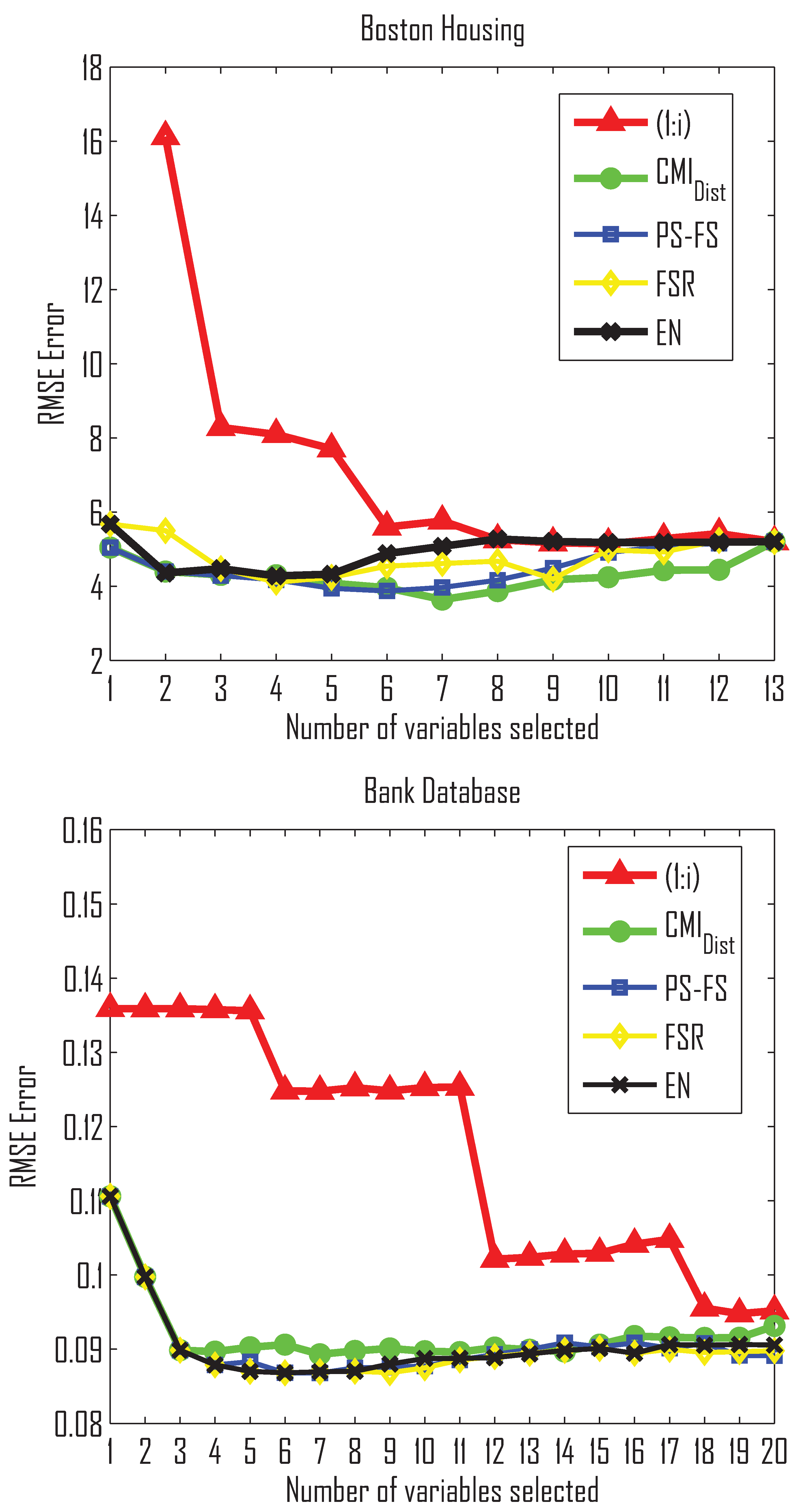
• In Table 3 we see that the proposed method $CM{I}_{Dist}$ obtains better performance with respect to the rest of methods for all the cases (5, 10, 15 and 20 variables) for the CASI-AHS-CHLOR and CASI-THERM datasets and for two out of the three (10 and 13 variables) for the Boston Housing dataset.
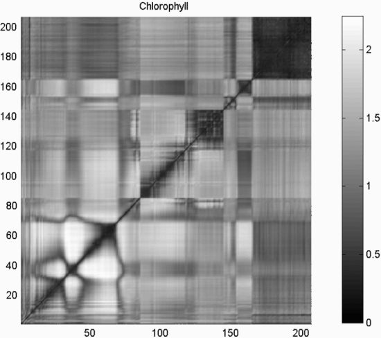
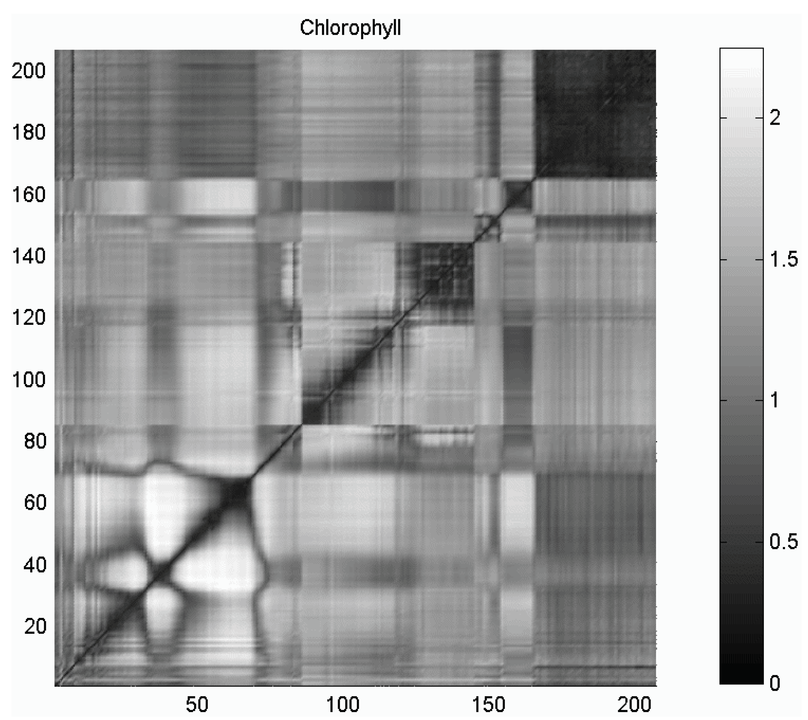
• In $CM{I}_{Dist}$ the clustering process plays an important role, which can be interpreted as a global strategy to obtain subsets of variables with high relevance in the estimation of the relevant variable Y obtained by the $\epsilon -$SVR algorithm. The dissimilarity space built from the conditional mutual information distances allows to find relationships between variables.
• The PS-FS method is the second best one in most cases followed by the EN method. PS-FS is a wrapper-type method based on a Neural Network regressor to make an optimal search where the error of the regressor acts as the search criteria.
• $FSR$ is the worst method in all the cases, with the exception of $K=10$ and $K=13$ for Boston Housing. For the Bank32NH dataset, all methods provide similar results.
• In two out of the four single-output regression datasets that appear in Table 3, when the dimension of the input variable space increases, the performance of the regression methods nevertheless decreases. One reason could be given by the Hughes phenomenon (the curse of dimensionality). Noise and variables considered as noisy may also degrade the quality of the regression.
• Table 4 shows the average RMSE over the four datasets for different sizes of the variable subsets selected. $CM{I}_{Dist}$ provides the best results for all cases, while the PS-FS method is the second best method.

Table 4. Average RMSE error over the four datasets and the first 5, 10, 15 and 20 variables. Boston Housing has 13 variables and it is not considered for the case of $K=20$.

Variables	${\mathit{CMI}}_{\mathbf{Dist}}$	PS−FS	FSR	EN
K = 5	2.691	2.745	3.275	2.877
K = 10	2.471	2.562	3.075	2.758
K = 15	2.451	2.543	2.995	2.705
K = 20	1.784	1.839	2.267	1.899

Table 4. Average RMSE error over the four datasets and the first 5, 10, 15 and 20 variables. Boston Housing has 13 variables and it is not considered for the case of $K=20$.

Variables	${\mathit{CMI}}_{\mathbf{Dist}}$	PS−FS	FSR	EN
K = 5	2.691	2.745	3.275	2.877
K = 10	2.471	2.562	3.075	2.758
K = 15	2.451	2.543	2.995	2.705
K = 20	1.784	1.839	2.267	1.899

The differences in RMSE ranked for the four methods are not significant for the first 5 variables, but they are significant when selecting 10 to 15 variables. Thus, the difference between the methods increases with the number of selected variables, although in the case of the CASI-THERM dataset the statistical tests suggests that there are not significant differences among the methods.

The selection of the first variable and the first two variables is better when using $CM{I}_{Dist}$ as compared to the rest of the methods. In this case, the clustering strategy plays an important role in the formation of different groups of variables, obtaining better results than a greedy selection algorithm as is the case of the FSR. In the case of the PS-FS and EN methods, the advantage of the $CM{I}_{Dist}$ method consists of a proper adjustment of the parameters from the Nadaraya-Watson function estimator and its use through a distance metric in the variable space that takes into account the internal relationships between variables.

4.2. Multi-Output Regression Datasets

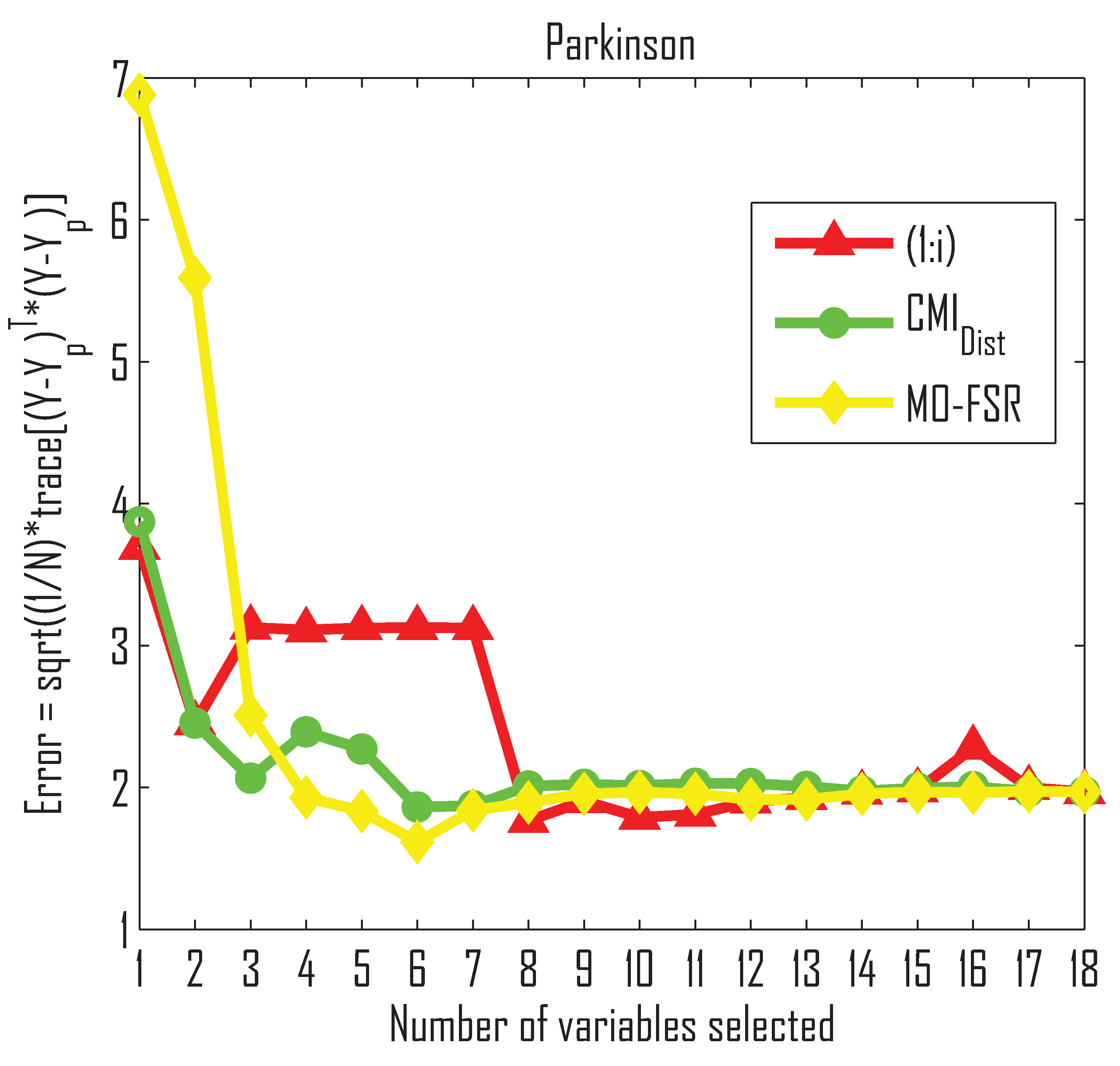
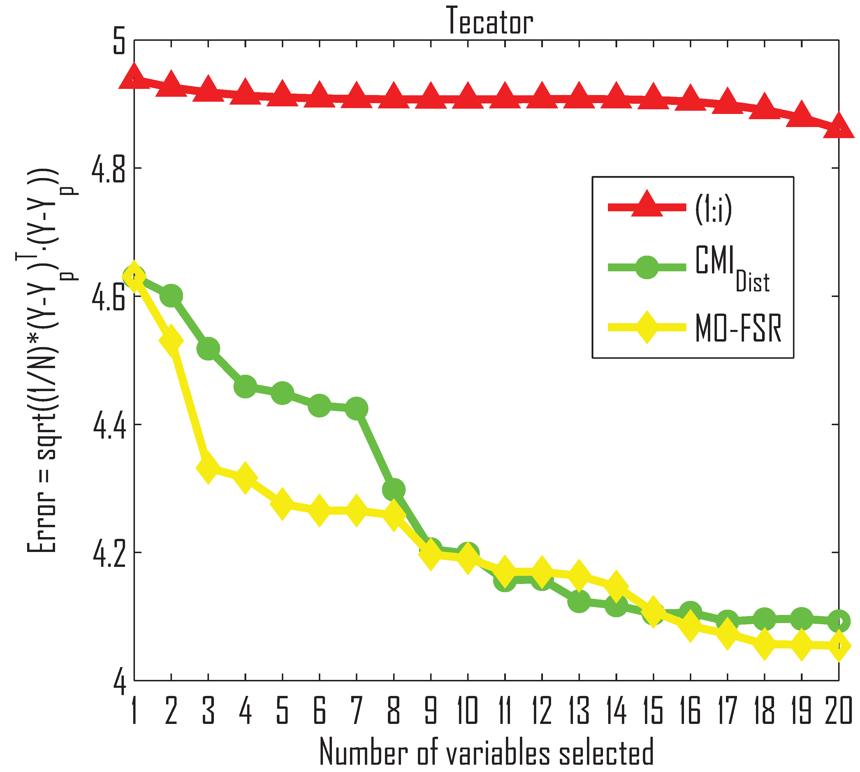
Sánchez et al. showed in [35] that SVR can be generalized to solve the problem of regression estimation for multiple (output) variables (hereafter, called MO-SVR). In fact, the use of a multidimensional regression tool helps in exploiting the dependencies between variables and makes the retrieval of each output variable less vulnerable to noise and measurement errors. Treating all the variables together may allow estimating each of them accurately if scarce data is available. The minimization of Equation (25) (Root-Mean Sum of Squares of the Diagonal, RMSSD) was used as a criterion to select the parameters of the MO-SVR regressor [38]:

$$RMSSD=\sqrt{\frac{1}{N}·trace({[\mathbf{Y}-{\mathbf{Y}}_p]}^T·[\mathbf{Y}-{\mathbf{Y}}_p])}$$

(25)

where ${\mathbf{Y}}_p$ is the output predicted matrix in the multi-output case, $\mathbf{Y}$ the corresponding original output matrix, trace is the trace of the matrix ${[\mathbf{Y}-{\mathbf{Y}}_p]}^T·[\mathbf{Y}-{\mathbf{Y}}_p]$ and N is the number of data points.

Figure 4 shows the RMSSD Error of the proposed method against the method by Kolar and Xing in [28]. Comparison results for different subsets of variables can be seen in Table 5. In this case, the Fisher distribution takes the values $F(1,4)=31.32$, $F(1,9)=13.61$, $F(1,14)=11.06$, and $F(1,19)=10.07$. The table shows the statistical significance as positive $(+)$ when the value of the test is greater than the Fisher distribution and negative $(-)$ otherwise. From Table 5, we can also see that:

• The $CM{I}_{Dist}$ method outperforms MO-FSR for the Parkinson dataset, while MO-FSR outperforms $CM{I}_{Dist}$ in the Tecator dataset. These experiments show that our method is comparable to MO-FSR.
• The $CM{I}_{Dist}$ method does not assume that the input and output data are linearly related, whereas MO-FSR does. Therefore, the performance of the selector may depend on the relationship between the input and output values for the datasets.
• The $CM{I}_{Dist}$ method outperforms MO-FSR for the first three selected variables in the Parkinson dataset, whereas there is no difference for the rest of the selected variables, as can be seen in the Friedman and Quade tests in Table 5. However, in the case of the Tecator dataset (see Figure 4b), the MO-FSR outperforms the $CM{I}_{Dist}$ up to variable 10, and tends to become equal afterwards.

Figure 4. Error for the Parkinson and Tecator multi-ouptut regression datasets.

Figure 4. Error for the Parkinson and Tecator multi-ouptut regression datasets.

Table 5. Average RMSSD Error over different subsets of original variables for the multi-output regression datasets.

Parkinson dataset
Variables	${\mathit{CMI}}_{\mathbf{Dist}}$	MO−FSR	Friedman Test	Quade Test
K = 5	2.611	3.749	0.17 (−)	0.87 (−)
K = 10	2.283	2.801	1.71 (−)	0.02 (−)
K = 15	2.191	2.515	7.87 (−)	1.18 (−)
K = 18	2.156	2.424	7.59 (−)	2.36 (−)
Tecator dataset
Variables	${\mathit{CMI}}_{\mathbf{Dist}}$	MO−FSR	Friedman Test	Quade Test
K = 5	4.531	4.417	7.11 (−)	9.92 (−)
K = 10	4.421	4.326	38.37 (+)	28.10 (+)
K = 15	4.325	4.268	1.07 (−)	3.80 (−)
K = 20	4.268	4.217	4.82 (−)	6.22 (−)

Table 5. Average RMSSD Error over different subsets of original variables for the multi-output regression datasets.

Parkinson dataset
Variables	${\mathit{CMI}}_{\mathbf{Dist}}$	MO−FSR	Friedman Test	Quade Test
K = 5	2.611	3.749	0.17 (−)	0.87 (−)
K = 10	2.283	2.801	1.71 (−)	0.02 (−)
K = 15	2.191	2.515	7.87 (−)	1.18 (−)
K = 18	2.156	2.424	7.59 (−)	2.36 (−)
Tecator dataset
Variables	${\mathit{CMI}}_{\mathbf{Dist}}$	MO−FSR	Friedman Test	Quade Test
K = 5	4.531	4.417	7.11 (−)	9.92 (−)
K = 10	4.421	4.326	38.37 (+)	28.10 (+)
K = 15	4.325	4.268	1.07 (−)	3.80 (−)
K = 20	4.268	4.217	4.82 (−)	6.22 (−)

5. Conclusions

This paper presents a filter-type variable selection technique for single and multi-output regression datasets, using a distance measure based on information theory. The main contributions of the paper are: (a) the variable selection method proposed in [11] for classification has been extended to single-output and multi-output regression problems involving selection of variables; (b) information theoretic criteria have been applied to extend the variable selection methodology to continuous variables; (c) a method to estimate the conditional entropy for single and multi-output continuous variables has been defined.

The proposed method outperforms the other methods used in the comparison in the case of single-output regression datasets, and it is also competitive in the case of the multi-output datasets considered. Therefore, the method proposed in this paper has a high generalization capability to apply the strategy to more than one output variable, because the conditional entropy can be directly extended for multivariate output datasets.

Variable selection in multi-output regression is a novel area of research that requires a deeper understanding in terms of the development of new selection techniques as well as in terms of the analysis of the inner structure of the datasets involved.

References

1. Dash, M.; Liu, H. Feature selection for classification. Intell. Data Anal. 1997, 1, 131–156. [Google Scholar] [CrossRef]
2. Verleysen, M.; Rossi, F.; Franois, D. Advances in feature selection with mutual information. Similarity Based Clust. 2009, 5400/2009, 52–69. [Google Scholar]
3. Karagiannopoulos, M.; Anyfantis, D.; Kotsiantis, S.B.; Pintelas, P.E. Feature selection for regression problems. In Proceedings of the 8th Hellenic European Research on Computer Mathematics & its Applications, Athens, Greece, 20–22 September 2007.
4. Oliveira, A.L.I.; Braga, P.L.; Lima, R.M.F.; Cornélio, M.L. GA-based method for feature selection and parameters optimization for machine learning regression applied to software effort estimation. Inf. Softw. Technol. 2010, 52, 1155–1166. [Google Scholar] [CrossRef]
5. Eirola, E.; Liitiäinen, E.; Lendasse, A. Using the delta test for variable selection. In Proceedings of the European Symposium on Artificial Neural Networks—Advances in Computational Intelligence and Learning, Bruges, Belgium, 23–25 April 2008; pp. 25–30.
6. Fan, J.; Peng, L.; Yao, Q.; Zhang, W. Approximating Conditional density functions using dimension reduction. Acta Math. Appl. Sin. 2009, 25, 445–456. [Google Scholar]
7. Rossi, F.; Lendasse, A.; Francois, D.; Wertz, V.; Verleysen, M. Mutual information for the selection of relevant variables in spectrometric nonlinear modelling. Chemom. Intell. Lab. Syst. 2006, 80, 215–226. [Google Scholar] [CrossRef]
8. Jain, A.K.; Duin, R.P.W.; Mao, J. Statistical pattern recognition: A review. IEEE Trans. Pattern Anal. Mach. Intell. 2000, 22, 4–37. [Google Scholar] [CrossRef]
9. Pudil, P.; Ferri, F.J.; Novovicova, J.; Kittler, J. Floating search methods for feature selection with nonmonotonic criterion functions. Pattern Recogn. 1994, 2, 279–283. [Google Scholar]
10. Caruana, R. Multitask learning. Mach. Learn. 1997, 28, 41–75. [Google Scholar] [CrossRef]
11. Sotoca, J.M.; Pla, F. Supervised feature selection by clustering using conditional mutual information-based distances. Pattern Recogn. 2010, 43, 2068–2081. [Google Scholar] [CrossRef]
12. Latorre Carmona, P.; Sotoca, J.M.; Pla, F.; Phoa, F.K.H.; Bioucas Dias, J. Feature selection in regression tasks using conditional mutual information. In Proceedings of the Iberian Conference on Pattern Recognition and Image Analysis (IbPRIA ’11), Las Palmas de Gran Canaria, Spain, 8–10 June 2011; pp. 224–231.
13. Ho, S.-W.; Verdu, S. On the interplay between conditional entropy and the error probability. IEEE Trans. Inf. Theory 2010, 56, 5930–5942. [Google Scholar] [CrossRef]
14. Cover, T.M.; Thomas, J.A. Elements of Information Theory; John Wiley & Sons Inc.: Hoboken, NJ, USA, 1991. [Google Scholar]
15. Peng, H.; Long, F.; Ding, C. Feature selection based on mutual information: Criteria of max-dependency, max-relevance, and min-redundance. IEEE Trans. Pattern Anal. Mach. Intell. 2005, 27, 1226–1238. [Google Scholar] [CrossRef] [PubMed]
16. Kwak, N.; Choi, Ch.-H. Input feature selection for classification problems. IEEE Trans. Neural Netw. 2002, 13, 143–159. [Google Scholar] [CrossRef] [PubMed]
17. Ward, J.H. Hierarchical grouping to optimize an objective function. J. Am. Stat. Assoc. 1963, 58, 236–244. [Google Scholar] [CrossRef]
18. Yeung, R.W. A First Course in Information Theory; Springer: Berlin, Heidelberg, Germany, 2002. [Google Scholar]
19. Ney, H. On the relationship between classification error bounds and training criteria in statistical pattern recognition. In Proceedings of the Iberian Conference on Pattern Recognition and Image Analysis (IbPRIA ’03), Puerto de Andratx, Mallorca, Spain, 4–6 June 2003; pp. 636–645.
20. Fan, J.; Yao, Q.; Tong, H. Estimation of conditional densities and sensitivity measures in nonlinear dynamical systems. Biometrika 1996, 83, 189–206. [Google Scholar] [CrossRef]
21. Hyndman, R.J.; Bashtannyk, D.M.; Grunwald, G.K. Estimating and visualizing conditional densities. J. Comput. Graph. Stat. 1996, 5, 315–336. [Google Scholar]
22. Holmes, M.P.; Gray, A.; Isbell, C.L. Fast kernel conditional density estimation: A dual-tree Monte Carlo approach. Comput. Stat. Data Anal. 2010, 54, 1707–1718. [Google Scholar] [CrossRef]
23. Rosenblatt, M. Remarks on some nonparametric estimates of a density function. Ann. Math. Stat. 1956, 27, 832–837. [Google Scholar] [CrossRef]
24. Nocedal, J.; Wright, S.J. Numerical Optimization, 2nd ed.; Springer: Berlin, Heidelberg, Germany, 2006. [Google Scholar]
25. Monteiro, S.T.; Kosugi, Y. Particle swarms for feature extraction of hyperspectral data. IEICE Trans. Inf. Syst. 2007, E90D, 1038–1046. [Google Scholar] [CrossRef]
26. Kennedy, J.; Eberhart, R. Particle swarm optimization. In Proceedings of the IEEE International Conference on Neural Networks, Perth, WA, Australia, 27 November–1 December 1995; pp. 1942–1948.
27. Zou, H.; Hastie, T. Regularization and variable selection via the elastic net. J. R. Stat. Soc. B 2005, 67, 301–320. [Google Scholar] [CrossRef]
28. Kolar, M.; Xing, E.P. Ultra-high dimensional multiple output learning with simultaneous orthogonal matching pursuit: Screening approach. In Proceedings of the International Conference on Artificial Intelligence and Statistics, Sardinia, Italy, 13–15 May 2010; pp. 413–420.
29. Obozinski, G.; Taskar, B.; Jordan, M.I. Joint covariate selection and joint subspace selection for multiple classification problems. Stat. Comput. 2010, 20, 231–252. [Google Scholar]
30. Moreno, J.F. SEN2FLEX Data Acquisition Report; Technical Report; Universidad de Valencia: Valencia, Spain, 2005. [Google Scholar]
31. DELVE data repository. Available online: http://www.cs.toronto.edu/∼delve/ (accessed on 15 February 2012).
32. Harrison, D.; Rubinfeld, D.L. Hedonic prices and the demand for clean air. J. Environ. Econ. Manag. 1978, 5, 81–102. [Google Scholar]
33. UCI machine learning repository. Available online: http://archive.ics.uci.edu/ml/ (accessed on 15 February 2012).
34. Drucker, H.; Burges, C.; Kaufman, L.; Kaufman, L.; Smola, A.; Vapnik, V. Support vector regression machines. In Neural Information Processing Systems; MIT Press: Cambridge, MA, USA, 1997; pp. 155–161. [Google Scholar]
35. Sánchez-Fernández, M.P.; de-Prado-Cumplido, M.; Arenas-García, J.; Pérez-Cruz, F. SVM multiregression for non-linear channel estimation in multiple-input multiple-output systems. IEEE Trans. Signal Process. 2004, 58, 2298–2307. [Google Scholar] [CrossRef]
36. Kwak, N.; Choi, Ch.-H. Input feature selection by mutual information based on parzen window. IEEE Trans. Pattern Anal. Mach. Intell. 2002, 24, 1667–1671. [Google Scholar] [CrossRef]
37. García, S.; Fernández, A.; Luengo, J.; Herrera, F. Advanced nonparametric tests for multiple comparisons in the design of experiments in computational intelligence and data mining: Experimental analysis of power. Inf. Sci. 2010, 180, 2044–2064. [Google Scholar] [CrossRef]
38. Johnson, R.A.; Wichern, D.W. Applied Multivariate Statistical Analysis; Prentice Hall: Upper Saddle River, NJ, USA, 2007. [Google Scholar]