Size Effects on the Entropy Production in Oscillatory Flow between Parallel Plates

Abstract

The heat transfer problem of a zero-mean oscillatory flow of a Maxwell fluid between infinite parallel plates with boundary conditions of the third kind is considered. The local and global time-averaged entropy production are computed, and the consequences of convective cooling of the plates are also assessed. It is found that the global entropy production is a minimum for certain suitable combination of the physical parameters and a discrete set of values of the separation between the parallel plates. The transferred heat at the plates also shows minima in the same discrete set of values of the plates separation.

1. Introduction

The design of many traditional heat removal engineering devices (such as heat exchangers and cooling modules) relies on heat transfer enhancement. The performance of real thermal devices for energy conversion processes is affected by irreversible processes that reduce their thermal efficiency. In fluid flow systems, the use of oscillatory flows has been investigated to improve transport processes in different situations. It has been found that oscillatory flows may enhance the transport mass compared to the molecular diffusive transport present in a motionless fluid [1]. The effective thermal diffusivity of a Newtonian fluid in a duct subjected to a zero-mean oscillatory flow may reach a maximum for a specific oscillation frequency and lead to heat transfer enhancement [2,3]. Moreover, in the case of a viscoelastic fluid flowing in a tube, the dynamic permeability may be enhanced at given resonant oscillation frequencies [4,5,6,7,8,9,10]. Oscillatory flows at high frequencies under conditions where inertial effects are negligible have also been studied in microfluidics applications [11]. In all these situations, the analysis of the entropy generation [12,13] has revealed as a tool for characterizing the associated irreversible processes, contributing to the enlightenment of the underlying physical processes and optimizing the performance of a given device. The physical mechanisms for size effects involve changes in the relative importance of various phenomena that determine the flow and heat transfer. Here stands the fact that the diminishing scale gives rise to surface-dominated effects. This results in variations of the friction factor, the heat transfer coefficient, the transition from laminar to turbulent flow, etc., and in general in the flow, heat transfer and entropy production regimes. In addition, when the characteristic length of the system becomes the same order of magnitude as the mean free path of the molecular components of the fluid, the continuum hypothesis breaks due to the rarefaction of the fluid under study. This situation will not be considered here in such a way that the velocity slip and the temperature jump at the boundaries are not included in the Navier-Stokes equations. Size effects have attracted the interest of both applied and theoretical researchers since several years ago [14,15,16,17,18,19,20,21]. In this paper we examine the size effects on the flow and heat transfer problem of a zero-mean oscillatory flow of a Maxwell fluid between infinite parallel plates with boundary conditions of the third kind. The emphasis is placed on the computation of the entropy generation [22] and the heat transfer in the plates. We will analyzed their dependence on the characteristic length represented by the distance between plates. We find that the global entropy production exhibits a series of maxima and minima for certain separation distances which had not been reported in the literature. The maxima are associated with maxima and minima of the heat being transferred at the plates. The relative importance of conductive and viscous loss processes and their relation with the entropy production is also determined. Our findings may shed some light on the factors affecting the physical behavior of oscillatory flows and, we hope, will provide additional useful information for designing thermal devices.

2. Transport Problem

2.1. Basic Assumptions

We consider the flow of a viscoelastic fluid between two infinite parallel plates separated by a distance $2a$. Specifically, we study an aqueous solution of cetylpyridinium chloride (CPyCl) and sodium salicylate (NaSal) which is modeled as a Maxwell fluid. Our results can be supported, in principle, by the fact that the Maxwell model constitutes a theoretical basis for the continuous description of viscoelastic fluids as the mentioned solution. See for example [23], where comparison of theoretical results with experiments was made with a good agreement. We assume that a zero-mean time-periodic pressure gradient is established in the system producing an oscillatory flow in the axial x-direction. With the former approximations, the flow becomes fully developed with all quantities depending on the transversal coordinate y and the time t, except for the pressure, which varies with x and t. We also assume that the fluid is incompressible and monocomponent, so that mass diffusion phenomena are disregarded. In addition, all physical properties of the fluid are assumed to be constant. Irreversible processes due to viscous stresses generate heat in the system and it exchanges heat with the surroundings through the Newton’s law of cooling. Finally, as a first approach we assume that the velocity slip and the temperature jump are not present at the plates containing the fluid.

2.2. Fundamental Equations

The continuity and momentum equations for this system are

$$\nabla ·\mathbf{u}=0$$

(1)

$$\rho \frac{\partial \mathbf{u}}{\partial t}+\left(\mathbf{u}·\nabla \right)\mathbf{u}=-\nabla p+\nabla ·\tau$$

(2)

where $\mathbf{u}$ and p , are the velocity and pressure fields while ρ and τ are the mass density and viscous stress tensor of the fluid. In turn, the heat transfer equation reads

$$\rho C_p\left(\frac{\partial T}{\partial t}+\left(\mathbf{u}·\nabla \right)T\right)=k{\nabla }^{2}T-\tau :\nabla \mathbf{u}$$

(3)

where T is the temperature, and $C_p$ and k are the specific heat at constant pressure and the thermal conductivity of the fluid, respectively. For the viscous stress tensor τ we consider the linear form of the Maxwell model, namely,

$$t_m\frac{\partial \tau }{\partial t}=-\eta \nabla \mathbf{u}-\tau$$

(4)

where η is the shear viscosity and $t_m$ the relaxation time for the Maxwell fluid. Note that if $t_m=0$ we recover the expression for the viscous stress tensor for the Newtonian fluid given by

$$\tau =-\eta \nabla \mathbf{u}$$

(5)

2.3. Velocity Field

Assuming an unidirectional flow that depends only on the transversal coordinate and time and using the equation for τ in the momentum balance equation yields

$$t_m\rho \frac{{\partial }^{2}u}{\partial t^2}+\rho \frac{\partial u}{\partial t}=-\left(1+t_m\frac{\partial }{\partial t}\right)\frac{\partial p}{\partial x}+\eta \frac{{\partial }^{2}u}{\partial y^2}$$

(6)

The oscillatory pressure gradient that produces the motion can be expressed as the real part of $(\partial p/\partial x)=G{e}^{i\omega t},$ where G is a constant. Therefore, we assume that the velocity is also a harmonic function of t, that is, $\mathbf{u}=\left[u=\frac{1}{2}\left(u_o\left(y\right)e^{i\omega t}+\overline{u_o\left(y\right)}{e}^{-i\omega t}\right),0,0\right]$, where the bar denotes complex conjugation. Under these circumstances the equation to be solved reads

$$\eta \frac{{\partial }^2{u}_0}{\partial y^2}=(1+i\omega t_m)(i\rho \omega u_0+G)$$

(7)

The corresponding non-slip boundary conditions for Equation (7) read $u_0(\pm a)=0.$ Though we take our analysis in the micro scales of length we do not use the slip boundary condition since the Knudsen number for the working fluid is $\le 0.001$. This condition is recognized [24,25] as the one which assures the validity of the continuous hypothesis for describing the transport phenomena in the system and it allows us to despise the slip of velocity at the plates. We calculate the Knudsen number through the expression

$${\kappa }_n=l/L$$

(8)

where l is the mean free path of the particles of the solution and L is a characteristic length which is taken to be the plate separation. The mean free path is obtained from a kinetic theory calculation [26] at a fluid particle concentration of 100 mM by taking the particle size of the fluid as 2.6 nm [23,27]. The value we obtain for the Knudsen number is $5.53\times {10}^{-4}$ for a plate separation of ${10}^{-3}$ m. The explicit (analytic) solution $u_0\left(y\right)$ of Equation (7), in terms of the parameters of the fluid and the separation $a,$ is given by

$$\begin{array}{ccc}\hfill u_0\left(y\right)& =& \frac{iG\left(-\right)\left(-i+\tau \omega \right)}{\rho \left(-i\omega +\tau {\omega }^2\right)}+\frac{i{e}^{a\sqrt{\rho \left(i\omega -\tau {\omega }^2\right)}G}}{\rho \omega \left(1+e^{2a\sqrt{\rho \left(i\omega -\tau {\omega }^2\right)}}\right)}\times (e^{-y\sqrt{\rho \left(i\omega -\tau {\omega }^2\right)}}-e^{y\sqrt{\rho \left(i\omega -\tau {\omega }^2\right)}})\hfill \end{array}$$

The average velocity $U_0$ is in turn given by

$$U_o=\frac{1}{2}{\int }_{-a}^{+a}{u}_{o}dy$$

(9)

2.4. Temperature Field

Once the velocity field is obtained, one may proceed to solve the energy balance equation. Here this equation is solved using boundary conditions of the third kind that indicate that the normal temperature gradient at any point in the boundary is assumed to be proportional to the difference between the temperature at the surface and the external ambient temperature. Hence, the amount of heat entering or leaving the system depends on the external temperature as well as on the convective heat transfer coefficient. The energy balance (3) for the Maxwell fluid may be written as

$$\rho C_p\frac{\partial T}{\partial t}=k\frac{{\partial }^{2}T}{\partial y^{*2}}+\frac{\eta }{{1+{\omega }^{2}t}_m^2}{\left(\frac{\partial u}{\partial y}\right)}^2$$

(10)

Note that the viscous dissipation contribution involves squared terms of harmonic functions of time. Consequently, the heat source term contains time harmonic terms with twice the frequency of oscillation as well as a steady contribution. Therefore, one may assume that the temperature has the form

$$T(y,t)=T_u\left(y\right)e^{2i\omega t}+\overline{T_u\left(y\right)}{e}^{-2i\omega t}+T_s\left(y\right)$$

(11)

where the sub-indexes u and s refer to the unsteady and steady contributions, respectively. Introducing Equation (11) into Equation (10), the equations satisfied by $T_u$, $\overline{T_u}$ and $T_s$ are found to be

$$k\frac{d^2{T}_u}{d{y}^2}-2i\rho C_p\omega T_u=-\frac{\eta }{4(1+{\omega }^2{t}_m^2)}{\left(\frac{\partial u_0}{\partial y}\right)}^2$$

(12)

$$k\frac{d^2\overline{T_u}}{d{y}^2}+2i\rho C_p\omega T_u=-\frac{\eta }{4(1+{\omega }^2{t}_m^2)}{\left(\frac{\partial \overline{u_0}}{\partial y}\right)}^2$$

(13)

and

$$k\frac{d^2{T}_s}{d{y}^2}=-\frac{1}{2(1+{\omega }^2{t}_m^2)}\left(\frac{\partial u_0}{\partial y}\right)\left(\frac{\partial \overline{u_0}}{\partial y}\right)$$

(14)

The solution to Equations (12)-(14) must satisfy the boundary conditions of the third kind, namely

$$k\frac{d{T}_s}{dy}+h_1\left(T{}_s-T_A\right)=0,\text{at}y=a$$

(15)

$$k\frac{d{T}_s}{dy}-h_2\left(T{}_s-T_A\right)=0,\text{at}y=-a$$

(16)

$$k\frac{d{T}_u}{dy}+h_1{T}_u=0,\text{at}y=a$$

(17)

$$k\frac{d{T}_u}{dy}-h_2{T}_u=0,\text{at}y=-a$$

(18)

where $T_A$ is the reference ambient temperature and $h_1$ and $h_2$ , the convective heat transfer coefficients of the lower and upper surfaces, respectively, which can be different. Apart from the spatial or the spatial and temporal dependence, such solutions are functions of ρ, $C_p$, $\eta ,$ $h_1$ , $h_2$ and $\omega .$ The expressions of the steady temperature $T_s\left(y\right)$ and the unsteady temperature $T_u\left(y\right)$ in terms of the parameters of the fluid and the separation a, numerically derived in this work with the aid of Mathematica from Equation (14) and its boundary conditions, will not be shown explicitly.

The velocity and temperature fields already obtained will be used for the determination of the entropy generation rate for this problem. The local entropy density generation rate, $\dot{S}$, that takes into account irreversible processes due to heat conduction and viscous losses is given by [9,10]

$$\dot{S}=\frac{k}{T{}^2}{\left(\frac{\partial T}{\partial y}\right)}^2+\frac{\eta }{T(1+{\omega }^2{t}_m^2)}{\left(\frac{\partial u}{\partial y}\right)}^2$$

(19)

Equation (19) is obtained from the Gibbs equation in conformity with the principles of irreversible thermodynamics (see [22] , Chapter 13). For the case of a constant density monocomponent fluid the Gibbs equation reduces to

$$T\frac{dS}{dt}=\frac{dU}{dt}$$

(20)

By introducing the balance equation of internal energy in the absence of electromagnetic fields an entropy balance equation is obtained where the entropy production takes the form

$$-\frac{1}{T^2}\mathbf{q}·\nabla T-\frac{1}{T}\tau :\nabla \mathbf{v}$$

(21)

being $\mathbf{q}$ the heat flux. If one introduces in the last expression the Fourier’s law and Equation (4) for the heat flux and the viscous stress tensor, respectively, one gets Equation (19).

Evidently, $\dot{S}$ is a function of space and time and, in fact, contains both time harmonic and steady parts. The global entropy generation rate per unit length in the axial direction, ${\dot{S}}_g$, is obtained by integrating $\dot{S}$ between the plates and over one period of time.

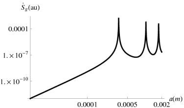
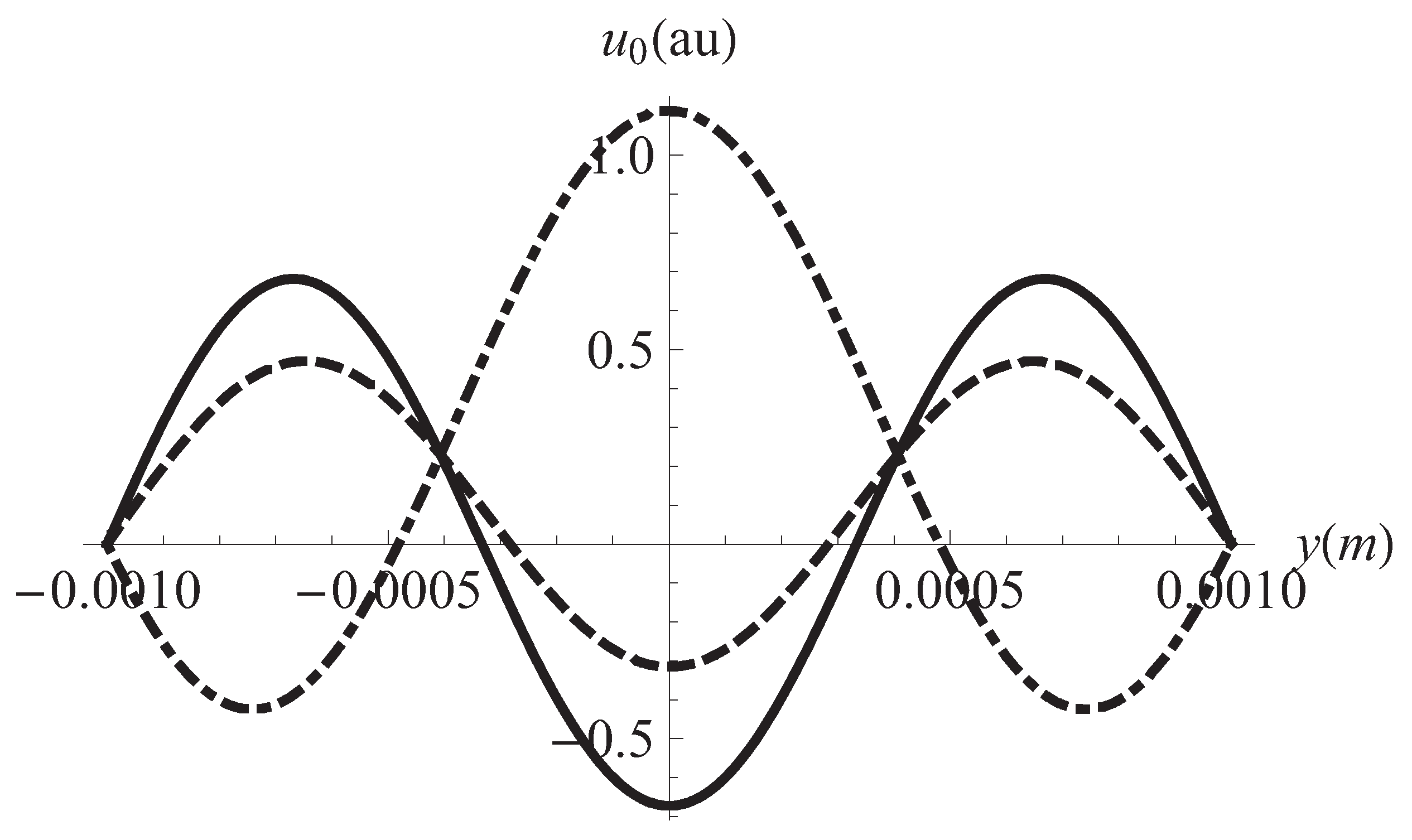
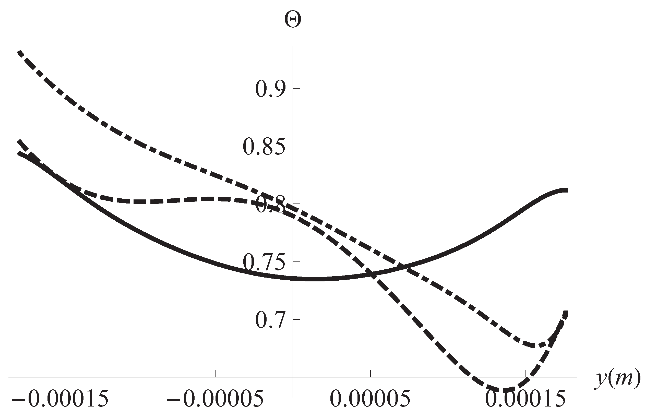
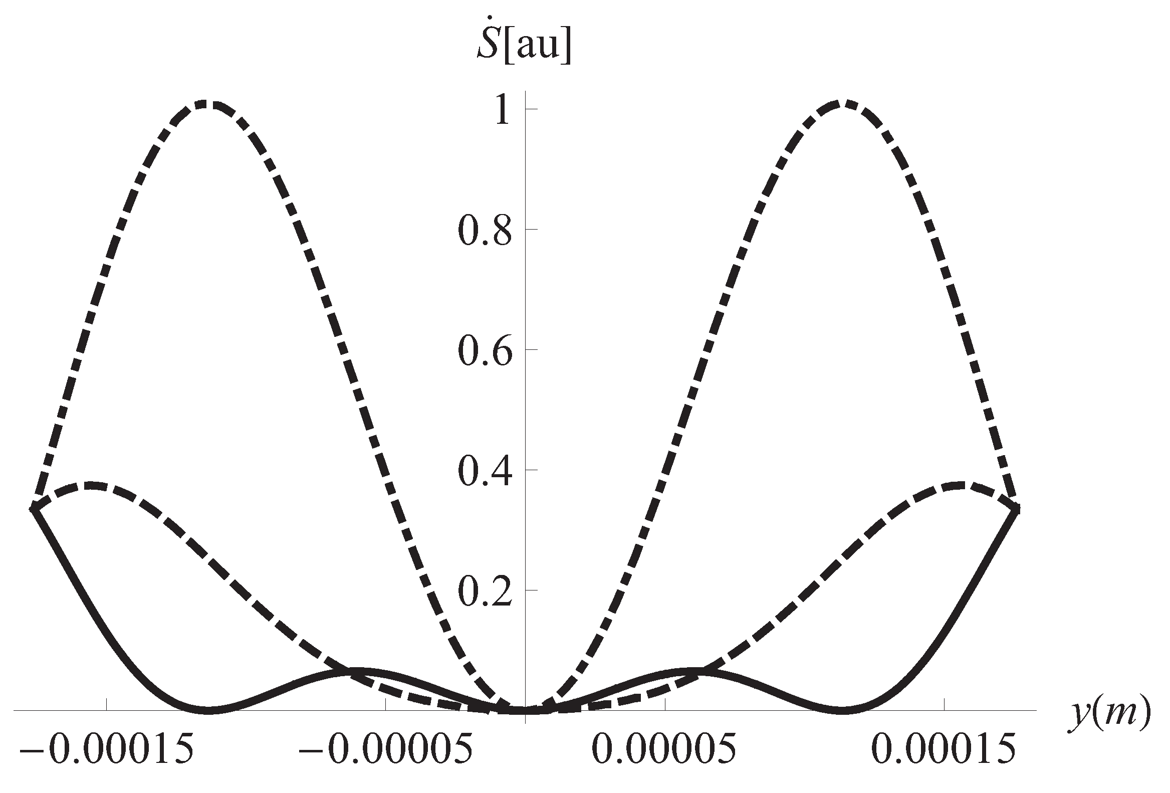
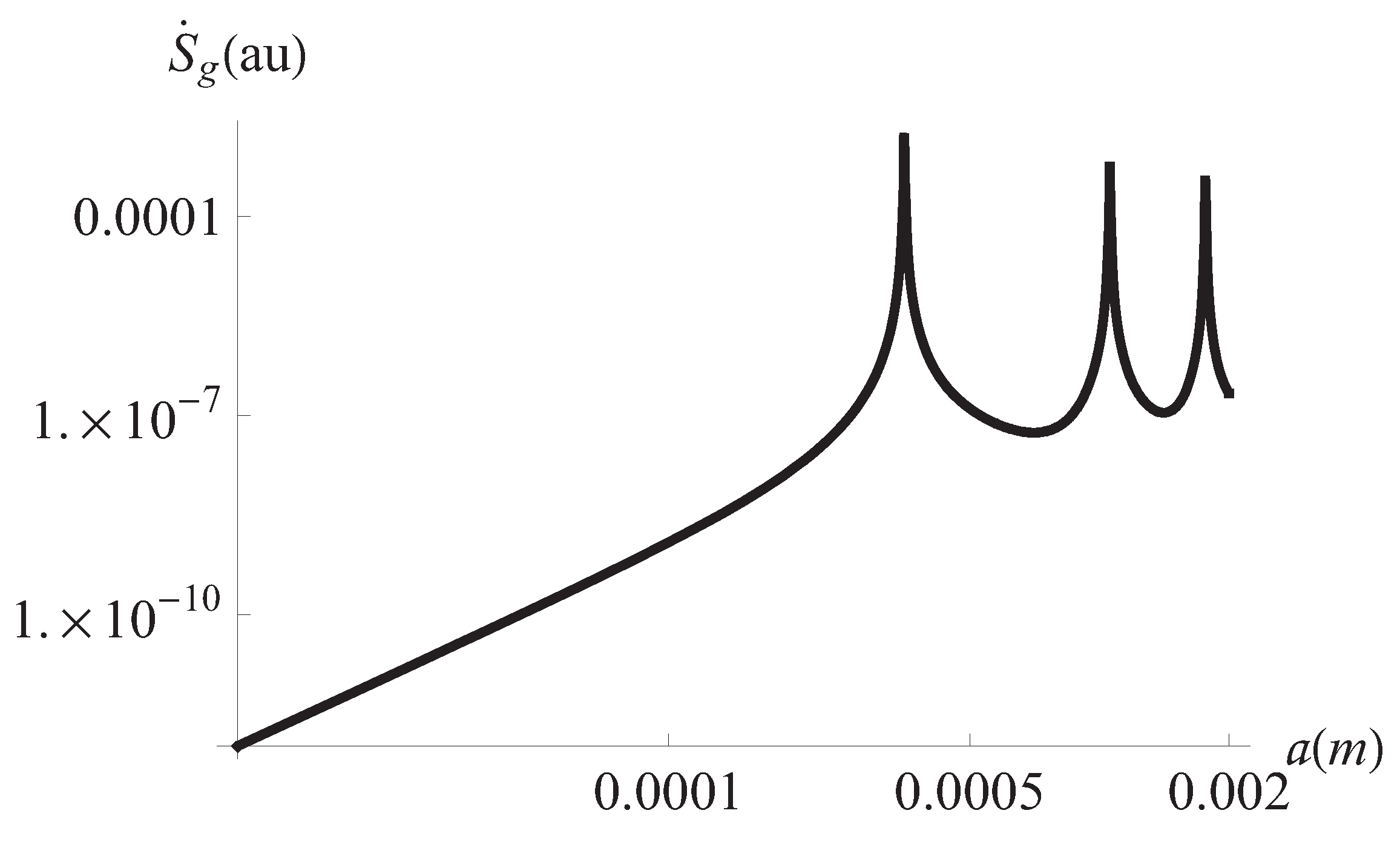
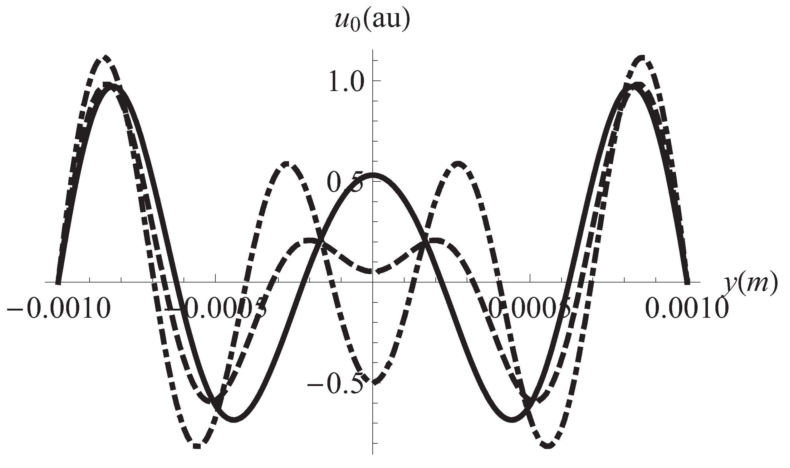
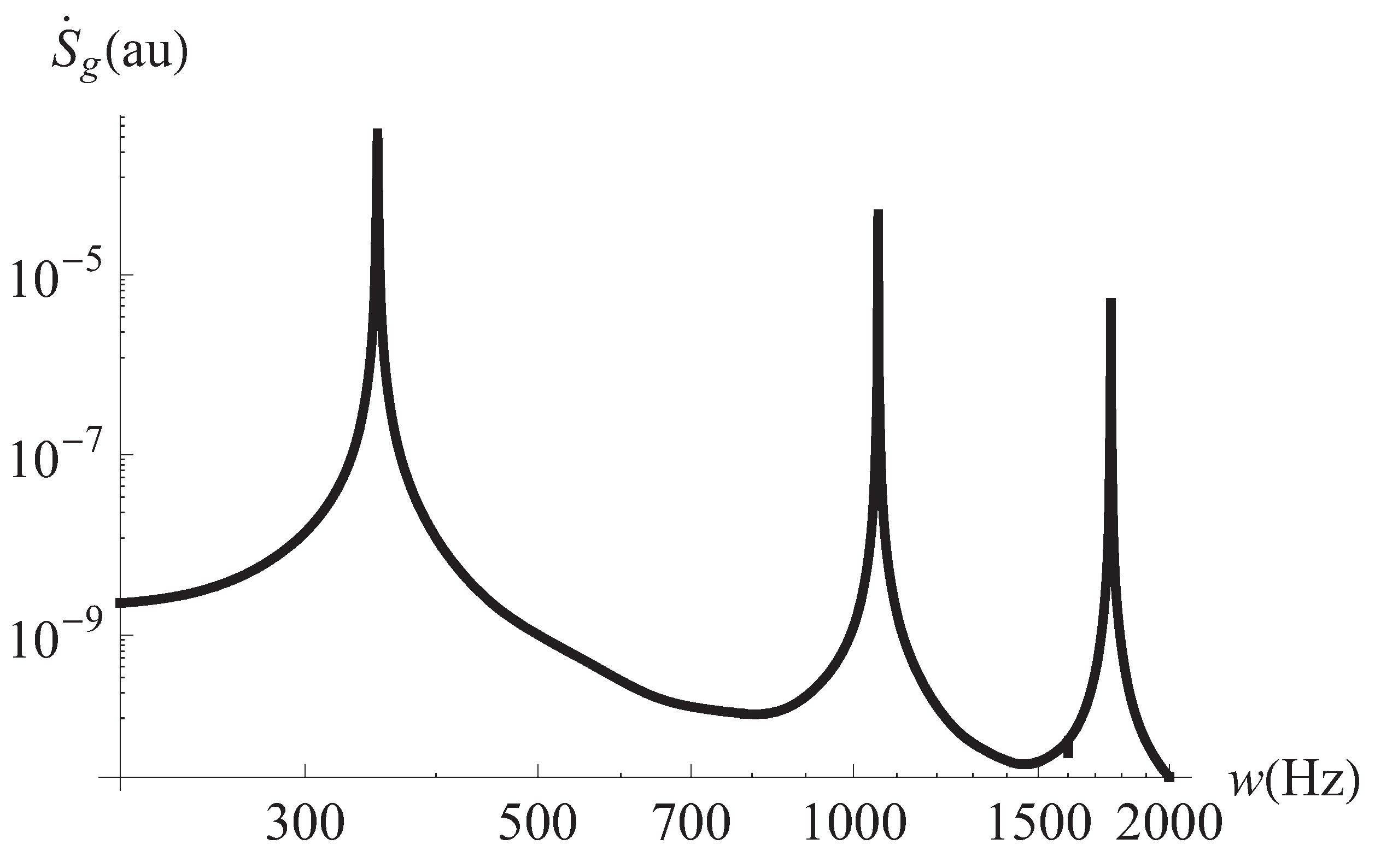
3. Results and Discussion

A particular choice of the values of the parameters defining the system was made in order to perform the further simulations. The values are the following: $k=0.58$ W/mK, $\rho =1050$ Kg/m${}^3$, $C_p=4.2\times {10}^3$ J/KgK and $\eta =60$ Pa s, $t_m=1.9$ s. The viscoelastic properties of this fluid correspond to an aqueous solution of cetylpyridinium chloride (CPyCl) 100 mM and sodium salicylate (NaSal) 60 mM [28]. The oscillation frequency ω in the pressure gradient was ranging from 100 Hz to $2\times {10}^3$ Hz and we took $T_A=300$ K. Finally, the separation between plates ranged from 100 μm to ${10}^{-3}$ m.

Firstly, Figure 1 and Figure 2 show the plot of $u_0$ as a function of the position along y axis for different times and frequencies of the applied external pressure gradient, respectively. Figure 3 corresponds to the profile of a normalized local temperature Θ along the y-coordinate for different times. The definition of Θ is as follows

$$\Theta \left(y,t\right)=\frac{T\left(y,t\right)-T_m}{T_{max}-T_{min}}$$

where $T_m$ is the mean temperature in the profile, $T_{max}$ and $T_{min}$ are the maximum and the minimum temperatures in the plot respectively.

Figure 1. Flux velocity vs. position in y for different times. Solid line: $t=0.00$ s, dashed: $t=2\times {10}^{-4}$ s, dotdashed: $t={10}^{-3}$ s. $\omega =100$ Hz, $a={10}^{-3}$ m.

We now consider the aim of this communication, namely, the study of the dependence of the entropy production and heat transfer on the plates separation. We begin with Figure 4 where the behavior of $\dot{S}$ with respect the position along y axis can be seen. The plot was obtained for three different times. Figure 5 shows one of the main results of this paper. The global entropy production, calculated by summing it on the profile along the y axis and over a period, shows maxima at certain values of the plates separation a. This is a remarkable result which will be commented below. We have calculated the Nusselt number which describes the relative importance of convective effects at the plates and found that it also has several maxima (Figure 6). These maxima coincide with those of the global entropy production shown in Figure 4 for the same values of the plates separation. The connection of this fact with the entropy generation will be discussed below too. It is convenient to introduce at this point the definition of the Nusselt number we have used in the calculation. The definition is the following [29,30]

$$Nu=\frac{-{\left(\frac{\partial T}{\partial y}\right)}_{y=\pm a}}{T_p-T_b}$$

(22)

being $T_p$ and $T_b$ the value of the temperature at the plate in $\pm a$ and the bulk temperature, respectively. This last defined as

$$T_b=\frac{\underset{-a}{\overset{a}{\int }}\rho T\left(y,t\right)u_0\left(y\right)dy}{\underset{-a}{\overset{a}{\int }}\rho u_0\left(y\right)dy}$$

Figure 2. Flux velocity vs. position in y for different frequencies of the external pressure gradient. Solid line: $\omega =200$ Hz, dashed: $\omega =210$ Hz, dotdashed: $\omega =220$ Hz. $a={10}^{-3}$ m.

Figure 3. Flux temperature vs. position in y for different times. Solid line: $t=0.0$ s, dashed: $t=0.2$ s, dotdashed: $t=0.4$ s. $a=1.7\times {10}^{-4}$ m, $h_1=5000$ J/m${}^2$K, $h_2=1000$ J/m${}^2$K.

Figure 4. Local entropy production vs. position in y for different times. Solid line: $t=0.00$ s, dashed: $t=2\times {10}^{-4}$ s, dotdashed: $t=3\times {10}^{-4}$ s. $\omega =100$ Hz, $a=1.7\times {10}^{-4}$ m.

Figure 5. Global entropy production vs. plates separation. $\omega =100$ Hz, $h_1=5000$ J/m${}^2$K, $h_2=1000$ J/m${}^2$K.

Figure 6. Nusselt number at upper plate vs. plates separation. $\omega =100$ Hz, $h_1=5000$ J/m${}^2$K, $h_2=1000$ J/m${}^2$K.

Finally, in Figure 7, the dependence of the entropy production can be found with respect to the frequency of the oscillation of the external pressure gradient. All the details of the mentioned figures can be found in the corresponding caption.

Figure 7. Global entropy production vs. frequency of the external pressure gradient. $a=0.0001$ m, $h_1=5000$ J/m${}^2$K, $h_2=1000$ J/m${}^2$K.

We begin the discussion of our results by remarking the effects of the viscoelastic properties of the working fluid. These properties reflect in Figure 1 and Figure 2 where it can be seen that different horizontal layers of the fluid flow with opposite velocities. This kind of behavior does not appear in the case of a Newtonian fluid [31]. It must be noted in Figure 3 the convective effects causing that the temperature at the plates differs from the reference temperature $T_A.$ Figure 4 displays the inhomogeneities of the local entropy generation in the profile along the y axis. Naturally, the maxima and minima in each case coincide with the maxima and minima shown by the velocity gradient in the profile. One of our main results is shown in Figure 5 where the maxima of ${\dot{S}}_g$ are periodically found in the considered range variation of the separation between the plates, namely, 10 μm to $2\times {10}^{-3}$ m. We have investigated the change of the conductive and viscous contribution to the entropy generation and the heat transfer at the plates with respect to the plates separation a in the same interval. First, we found that viscous dissipation becomes the most important contribution dominating heat conductive effects in that interval. So, the main internal heat source in the system is the shearing of fluid layers. This is characteristic of the surface-dominated phenomena in small scale devices [16]. For $a\ge 2\times {10}^{-3}$ m viscous losses and conductive contributions become comparable in magnitude. Our calculations showed that the maxima of the global entropy generation are due mainly to the presence of maxima in the dissipative viscous contribution. The physical mechanism of this amplification for certain values of a is to be determined. The position of the maxima with respect to the separation a depends only on the frequency of the external pressure gradient. The position is not affected by other physical parameters. The intensity G of the external gradient only increases the value of the global entropy production without changing the position of the maxima. Our finding was that the position of the maxima moves towards smaller values of a as the frequency is increased. This would imply, in principle, that in the high frequency operation the maxima in the global entropy generation may appear when the plates separation is of the order of magnitude of nanometers. This is an interesting conclusion for the design of nanodevices which deserves more investigation by applying the proper boundary conditions. In relation to the heat transfer at the plates, Figure 6 shows the corresponding result of this study. The relative importance of convective effects at the plates was calculated through the Nusselt number as defined in Equation (22). It was found that the Nusselt number also has maxima at the same values of the separation between plates where the entropy generation has maxima. In turn, these maxima coincide with the maxima of the conductive and viscous contributions to the entropy production. Here it must be mentioned again the tendency of the maxima in the Nusselt number to move towards smaller values of the separation between the plates as the oscillation frequency increases. Translating the previous comments to temperature gradient at the plates language, it should be stressed that it increases its magnitude when the convective coefficients $h_1$ or $h_2$ are increased. All our graphs were obtained with $h_1$ (upper plate) $<h_2$ (lower plate). In Figure 6 we have shown the upper plate case ($y=a$) so in the lower plate case we should expect the presence of minima (in fact negative minima) at the same values of the plates separation with an absolute value bigger than those maxima in the upper plate case. The sign of the temperature gradient at the plates indicates that heat is transferred from the outside into the system in both cases. Nevertheless, it is worth noting that if $h_1\ll h_2$ then both extremes have positive values. This indicates that heat is being transferred from the outside of the upper plate to the outside of the lower plate. Finally, in Figure 7 it can be seen that the global entropy production also has maxima when the frequency is varied for a fixed value of the separation between the plates. This allows one to infer the dependence of the global entropy production on the oscillatory Reynolds number $R_{\omega }$ defined as

$$R_{\omega }=\frac{\rho \omega a^2}{\eta }$$

(23)

Expression (23) implies that the plot ${\dot{S}}_g$ vs. $R_{\omega }$ has the same shape as that of the plot ${\dot{S}}_g$ vs. ω shown in Figure 7.

4. Summary and Conclusions

In this work we have analyzed the problem of an oscillatory flow of a Maxwell fluid between infinite parallel plates and considered the effects of the separation between the plates with boundary conditions of the third kind. After deriving the velocity and temperature fields, we computed the local and global entropy production in the system. It has been found that the global entropy generation shows maxima at specific values of the separation between the parallel plates. Two facts accompany the appearance of these maxima in the global entropy production. On the one hand, the conductive and viscous dissipative contributions to the entropy production in the bulk also show maxima at the same values of the separation between the plates. On the other, the heat transferred in the plates has maxima at those values of a too. The system can be operated in such a way that heat can be transferred at big rates from the lower to the upper part of the device. As the frequency of the oscillatory external pressure gradient is increased, the maxima appear for smaller separation values and eventually they appear in the microscale and even in the nanoscale of lengths.

It can be concluded that for a suitable combination of geometric design, physical parameters involved in the oscillatory regime of the problem and those defining the boundary conditions, the system can operate in a minimum global entropy production state avoiding the most dissipative working conditions, but they can be combined to get the maximum rate of heat transferred from the upper part to the lower part of the device (or vice versa). The role played by the separation between the parallel plates must be specially remarked. This can be a useful information for designing thermal devices.

References

1. Chatwin, P.C. On the longitudinal dispersion of passive contaminant in oscillating flows in tubes. J. Fluid Mech. 1975, 71, 513–527. [Google Scholar] [CrossRef]
2. Kurzweg, U.H. Enhanced heat conduction in fluids subjected to sinusoidal oscillations. J. Heat Transfer 1985, 107, 459–462. [Google Scholar]
3. Kurzweg, U.H. Enhanced heat conduction in oscillating viscous flows within parallel-plate channels. J. Fluid Mech. 1985, 156, 291–300. [Google Scholar] [CrossRef]
4. López de Haro, M.; del Río, J.A.; Whitaker, S. Transport Porous Media 1996, 25, 167.
5. del Río, J.A.; López de Haro, M.; Whitaker, S. Enhancement in the dynamic response of a viscoelastic fluid flowing in a tube. Phys. Rev. E 1998, 58, 6323–6327. [Google Scholar] [CrossRef]
6. del Río, J.A.; López de Haro, M.; Whitaker, S. Erratum: Enhancement in the dynamic response of a viscoelastic fluid flowing in a tube. Phys. Rev. E 2001, 64, 039901. [Google Scholar] [CrossRef]
7. Tsiklauri, D.; Beresnev, I. Enhancement in the dynamic response of a viscoelastic fluid flowing through a longitudinally vibrating tube. Phys. Rev. E 2001, 63, 046304–046308. [Google Scholar] [CrossRef]
8. Castrejón-Pita, J.R.; del Río, J.A.; Castrejón-Pita, A.A.; Huelsz, G. Experimental observation of dramatic differences in the dynamic response of Newtonian and Maxwellian fluids. Phys. Rev. E 2003, 68, 046301–046305. [Google Scholar] [CrossRef]
9. Lambert, A.A.; Ibáñez, G.; Cuevas, S.; del Río, J.A. Optimal behavior of viscoelastic flow at resonant frequencies. Phys. Rev. E 2004, 70, 056302. [Google Scholar] [CrossRef]
10. Lambert, A.A.; Ibáñez, G.; Cuevas, S.; del Río, J.A. Erratum: Optimal behavior of viscoelastic flow at resonant frequencies. Phys. Rev. E 2006, 73, 049902. [Google Scholar]
11. Yakhot, V.; Colosqui, C. Stokes’ second flow problem in a high-frequency limit: Application to nanomechanical resonators. J. Fluid Mech. 2007, 586, 249–258. [Google Scholar] [CrossRef]
12. Bejan, A. Entropy Generation through Heat and Fluid Flow; Wiley: New York, NY, USA, 1994. [Google Scholar]
13. Bejan, A. Minimization of Entropy Generation; CRC Press: Boca Raton, FL, USA, 1996. [Google Scholar]
14. Sobhan, Ch.B.; Garimella, S.V. A comparative analysis of studies on heat transfer and fluid flow in microchannels. Microscale Thermophys. Eng. 2001, 5, 293–311. [Google Scholar] [CrossRef]
15. Guo, Z.-Y.; Li, Z.X. Size effects on microscale single-phase flow and heat transfer. Int. J. Heat Mass Tran. 2003, 46, 149–159. [Google Scholar] [CrossRef]
16. Guo, Z.-Y.; Li, Z.X. Size effects on single-phase channel flow and heat transfer at microscale. Int. J. Heat Fluid Flow 2003, 24, 284–298. [Google Scholar] [CrossRef]
17. Morini, J.L. Single-phase convective heat transfer in microchannels: A review of experimental results. Int. J. Therm. Sci. 2004, 43, 631–651. [Google Scholar] [CrossRef]
18. Bayraktar, T.; Pidugu, S.B. Characterization of liquid flows in microfluidic systems. Int. J. Heat Mass Tran. 2006, 49, 815–824. [Google Scholar] [CrossRef]
19. Hooman, K. Entropy generation for microscale forced convection: Effects of different thermal boundary conditions, velocity slip, temperature. Int. Comm. Heat Mass Tran. 2007, 34, 945–957. [Google Scholar] [CrossRef]
20. Liang, X. Some effects of interface on fluid flow and heat transfer on micro- and nanoscale, jump, viscous dissipation, and duct geometry. Chin. Sci. Bull. 2007, 52, 2457–2472. [Google Scholar] [CrossRef]
21. Yao, J.; Yao, Y.F.; Patel, M.K.; Mason, P.J. On Reynolds number and scaling effects in microchannel flows. Eur. Phys. J. Appl. Phys. 2007, 37, 229–235. [Google Scholar] [CrossRef]
22. de Groot, S.R.; Mazur, P. Non-Equilibrium Thermodynamics; Dover: New York, NY, USA, 1984. [Google Scholar]
23. Fischer, P.; Rehage, H. Non-linear flow properties of viscoelastic surfactant solutions. Rheol. Acta 1997, 36, 13–27. [Google Scholar] [CrossRef]
24. Aydin, O.; Avci, M. Analysis of laminar heat transfer in micro-Poiseuille flow. Int. J. Therm. Sci. 2007, 46, 30–37. [Google Scholar] [CrossRef]
25. Beskok, A.; Karniadakis, G.E. Simulation of heat and momentum transfer in complex micro-geometries. J. Thermophys. Heat Tran. 1994, 8, 355–370. [Google Scholar] [CrossRef]
26. Reichl, L. A Modern Course in Statistical Physics; John Wiley & Sons, Inc.: New York, NY, USA, 1998; Chapter 11. [Google Scholar]
27. Oelschlaeger, C.; Schopferer, M.; Scheffold, F.; Willenbacher, N. Linear-to-branched micelles transition: A rheometry and diffusing wave spectrometry (DWS) study. Langmuir 2009, 25, 716–723. [Google Scholar] [CrossRef] [PubMed]
28. Rehage, H.; Hoffman, R.H. Rheological properties of viscoelastic surfactant systems. J. Phys. Chem. 1988, 92, 4712–4719. [Google Scholar] [CrossRef]
29. Ibáñez, G.; Cuevas, S.; López de Haro, M. Minimization of entropy generation by asymmetric convective cooling. Int. J. Heat Mass Tran. 2003, 46, 1321–1328. [Google Scholar] [CrossRef]
30. Ibáñez, G.; Cuevas, S.; López de Haro, M. Thermodynamic optimization of radial MHD flow between parallel circular disks. J. Non-Equilib. Thermodyn. 2004, 29, 107–122. [Google Scholar]
31. Vázquez, F.; Olivares-Robles, M.A.; Cuevas, S. Viscoelastic effects on the entropy production in oscillatory flow between parallel plates with convective cooling. Entropy 2009, 11, 4–26. [Google Scholar] [CrossRef]