Article

Multi-Criteria Evaluation of Energy Systems with Sustainability Considerations

1
School of Naval Architecture and Marine Engineering, National Technical University of Athens, Heroon Polytechniou 9, 157 80 Zografou, Greece
2
Athanasiou Krinou 10, 84 100 Ermoupoli, Syros, Greece
*
Author to whom correspondence should be addressed.
Entropy 2010, 12(5), 1006-1020; https://doi.org/10.3390/e12051006
Submission received: 25 February 2010 / Revised: 8 March 2010 / Accepted: 23 April 2010 / Published: 27 April 2010
(This article belongs to the Special Issue Exergy: Analysis and Applications)

Abstract

:
A multi-criteria approach is presented for the assessment of alternative means for covering the energy needs (electricity and heat) of an industrial unit, taking into consideration sustainability aspects. The procedure is first described in general terms: proper indicators are defined; next they are grouped in order to form sub-indices, which are then used to determine the composite sustainability index. The procedure is applied for the evaluation of three alternative systems. The three systems are placed in order of preference, which depends on the criteria used. In addition to conclusions reached as a result of the particular case study, recommendations for future work are given.

1. Introduction

In 1987 the document known as “the Brundtland Report” was published, raising the concern about sustainable development and introducing the definition of sustainability as the way to meet the needs of the present without compromising the ability of future generations to meet their own needs [1]. The three pillars of sustainability are the environmental performance, the social responsibility and the economic contribution, also called the “triple bottom line” concept.
As noted by Lior [2], “While providing an ethical and sensible direction, it is obvious that it is very difficult to quantify (sustainability), since it does not define what the current needs are, what the composition of future generations is, what their needs should be, which resources they would use, what the availability of these resources would be, and what the time frame is. Quantification of sustainability is a vital first step in human attempt to attain it, and in establishing the critically needed sustainability science.
The difficulty to quantify sustainability explains: (i) why many publications present sustainability in qualitative terms only, and (ii) why different groups of persons (policy makers, social scientists, economists, engineers, etc.) specify different sets of sustainability indicators that fit the particular type of application. A brief review of sustainability metrics (or indicators) as applied to energy issues is presented in [2].
The performance evaluation and (design and/or operation) optimization of energy conversion systems is usually based on single criteria (efficiency, cost, etc.). In the work presented in the following, which is extracted from [3] and further elaborated, a multi-criteria approach is followed that builds on the concept of sustainability. It is recognized that the list of criteria used is far from complete; therefore this is only a first step that needs to be taken further.

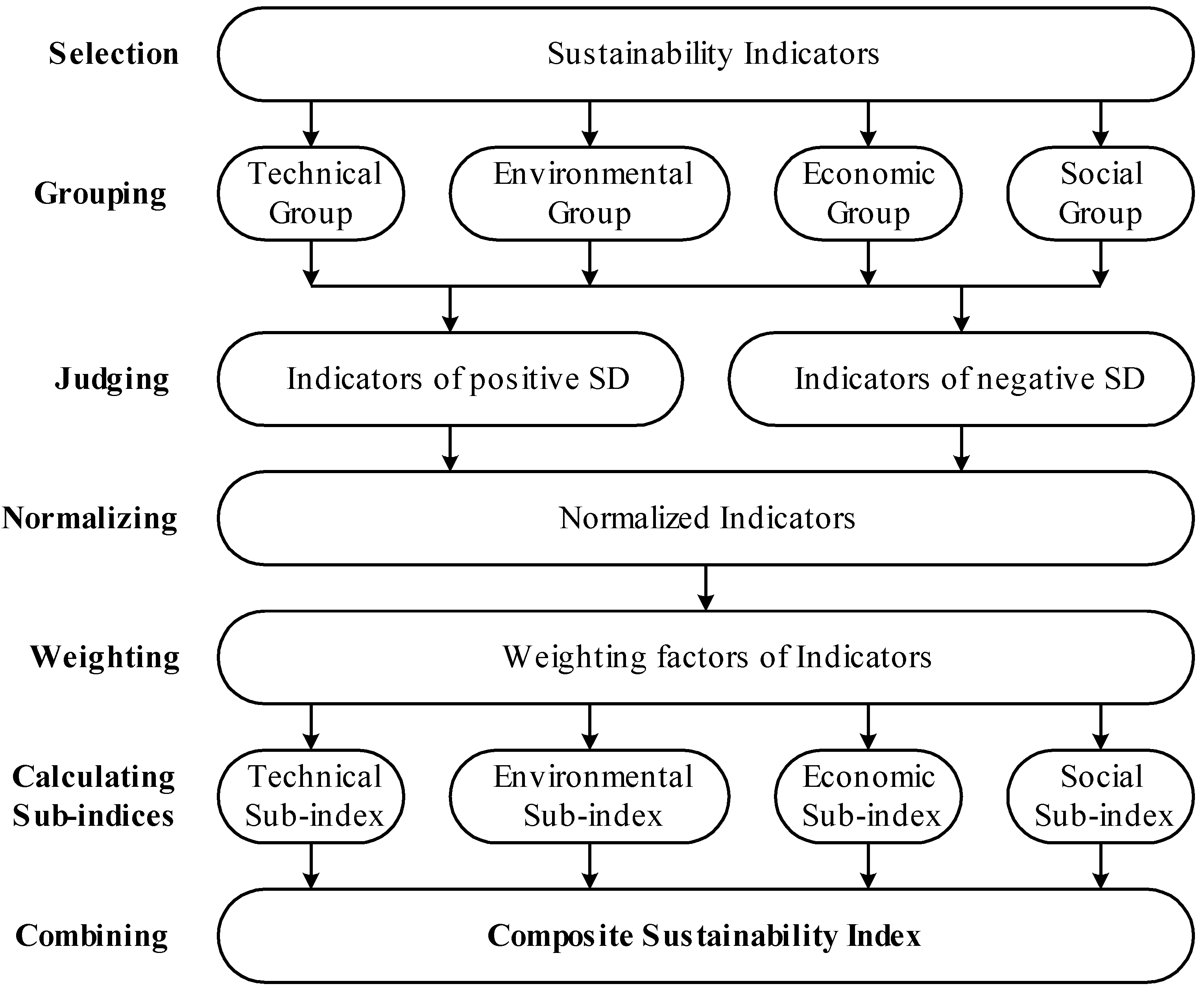
2. From Sustainability Indicators to Composite Sustainability Index

There are numerous indicators that can be used to assess the performance of an energy conversion system [2,4,5]. Each indicator reveals a certain aspect of the system performance, which is important. However, it may be difficult to make decisions as to, e.g., which of the options available is preferable from the sustainability point of view, based on a large number of indicators. For this purpose, sub-indices and a composite index are helpful. The aggregation of different indicators into a properly constructed index is not something trivial and many approaches can be followed. Here, a variation of the methods described in [4,6] is applied. The procedure is described in the following and depicted in Figure 1.

2.1. Selection and Grouping of Indicators

The first step is to select proper performance indicators reflecting different aspects of sustainability. There may be aspects of sustainability that can be only qualitatively described (e.g., certain social aspects), but for the assessment of energy systems every possible effort should be made to define quantitative indicators.
The concept of three pillars mentioned in the Introduction is extended in the case of energy systems to four pillars: technical, environmental, economic and social. Thus, it facilitates the evaluation, if the indicators are classified in four groups:
  • Technical indicators (energetic efficiency, exergetic efficiency, power density, fuel consumption, reliability, availability, etc.)
  • Environmental indicators (quantities of emitted pollutants, effect on health, effect on flora and fauna, etc.)
  • Economic indicators (life cycle cost, internal rate of return, payback period, etc.)
  • Social indicators (job creation, general welfare, etc.).
The indicator i of group j will be symbolized with I i j . The groups will be numbered in the order they are mentioned above (technical: j = 1, environmental: j = 2, economic: j = 3, social: j = 4).
Figure 1. Steps for calculation of composite sustainability index (adapted from [6]).
Entropy 12 01006 g001

2.2. Judging the Indicators

For certain indicators (e.g., efficiency), an increasing value reflects a positive effect on sustainability (“more is better”). For other indicators (e.g., emission of pollutants), an increasing value reflects a negative effect on sustainability (“less is better”). A judgment of the indicators in each group from this point of view will facilitate the analysis, as it will be shown in the following subsection.

2.3. Normalizing the Indicators

The indicators may be expressed in different units and consequently they cannot be used in their initial form for the calculation of the sub-indices and of the composite sustainability index. For this purpose, there is need of normalization. Even though more elaborate techniques can be found, for the purposes of this work it is suitable to normalize the indicators as follows.
For an indicator of the type “more is better”:
I ¯ i j = { 0 i f   I i j a i j I i j a i j b i j a i j i f   a i j < I i j < b i j 1 i f   I i j b i j
For an indicator of the type “less is better”:
I ¯ i j = { 1 i f   I i j a i j b i j I i j b i j a i j i f   a i j < I i j < b i j 0 i f   I i j b i j
In Equations (1) and (2), a i j is the lower threshold or limit of I i j , b i j is the upper threshold or limit of I i j , and I ¯ i j is the normalized indicator corresponding to I i j . According to their definition, all normalized indicators are non-dimensional.

2.4. Weighting the Indicators and Calculating the Sub-Indices

It is desirable to calculate a sustainability sub-index for each group of indicators, taking into consideration the importance of each indicator. However, it is difficult, if at all possible, to determine with sufficient accuracy the individual importance of each indicator. Therefore, pair-wise comparison has been introduced in the literature [6,7], which leads to relative weights of indicators. Using this technique, the Sustainability Sub-index of group j, I ¯ S j , is determined by the equation:
I ¯ S j = i w i j I ¯ i j
where w i j is the relative weight of indicator i in group j of indicators, defined in such a way that the following equation is satisfied:
i w i j = 1 ,    w i j 0

2.5. The Composite Sustainability Index

The procedure used in the preceding subsection to determine the sub-indices, is used also to determine the composite sustainability index, I C S :
I C S = j w j I ¯ S j
where w j is the relative weight given to the group j of indicators, defined in such a way that the following equation is satisfied:
j w j = 1 ,    w j 0
These weights reflect the importance given to the technical, environmental, economic and social performance of a system.

3. Case Study: Assessment of Alternative Energy Systems Related to An Industrial Unit

The procedure described in the preceding section is applied here in order to assess the performance of alternative means for covering the energy needs (electrical and thermal energy) of an industrial unit.

3.1. Selection of Indicators

The indicators defined in Table 1 are selected.
Table 1. Indicators for evaluation of alternative systems.
iSymbolUnitsDescription
1 η e Energetic electric efficiency
2 η t o t Energetic total efficiency
3 ζ e Exergetic electric efficiency
4 ζ t o t Exergetic total efficiency
5 m N O x kg/aAnnual emission of NOx
6 m C O kg/aAnnual emission of CO
7 m U H C kg/aAnnual emission of UHC (unburned hydrocarbons)
8 m P M 10 kg/aAnnual emission of PM10 (particular mater of a diameter up to 10 μm)
9 m C O 2 kg/aAnnual emission of CO2
10 m S O x kg/aAnnual emission of SOx
11NPCNet Present Cost (conventional analysis)
12NPCenvNet Present Cost including environmental externalities
It is recognized that these indicators belong to three groups: technical (i = 1–4), environmental (i = 5–10) and economic (i = 11–12). Unfortunately, due to lack of sufficient data, it has not been possible to include social indicators in the analysis.

3.2. Energy Needs of the Industrial Unit and Alternative Energy Systems

A steady state operation of the industrial unit is considered that requires electric power and saturated steam as specified in Table 2 (taken purposefully from [8,9], with certain adaptations).
Table 2. Energy needs of the industrial unit.
Electric power: W ˙ = 30000 kW
Mass flow rate of saturated steam: m ˙ s = 14 kg/s
Steam pressure: p = 20 bar
Feed water properties: p = 20 bar,  T = 25 °C
Annual operation: τ = 7480 h (11 months/a × 680 h/month)
Three alternative systems are considered for covering the aforementioned needs:
System A:
Electricity from the local network and steam from a boiler operating with natural gas and located in the industrial unit.
System B:
Gas turbine cogeneration system operating with natural gas, as the one described in the CGAM Problem [8,9].
System C:
Cogeneration system with dual fuel reciprocating internal combustion engine.
Values of the parameters common to all three alternatives are given in Table 3.
Table 3. Data common to Systems A, B and C.
Lower heating value of natural gas: H u N G = 36400 kJ/Nm3
Temperature of the environment:T0 = 25 °C (298.15 K)
Exergy to energy ratio of natural gas: ϕ N G = 1.04
Technical life of the system: N = 20 years
Salvage value at the end of N years: V s N = 0
Cost of natural gas: c N G = 0.2 €/Nm3
Market interest rate:i = 0.10
General inflation rate:f = 0.03
Fuel inflation rate:ff = 0.04
Annual insurance rate: Δ i n s = 0.5 % of investment
The heat flow rate required by the industrial unit and its exergy content are calculated with the equations:
Q ˙ = m ˙ s ( h s h w )    E ˙ s Q = m ˙ s [ h s h w T 0 ( s s s w ) ]
The specific enthalpy (h) and entropy (s) of feed water and saturated steam for the properties given in Table 2 are obtained from steam tables, while T0 is given in Table 3. The results are as follows:
Q ˙ = 37668   kW    E ˙ s Q = 12747.5   kW
Specific emissions (mass of pollutant per kWh) have been adapted from [10], taking into consideration that the efficiencies of the systems examined here are different from the efficiencies considered in [10] and assuming that the quantity of each emitted pollutant is inversely proportional to the efficiency of a plant. Values for the external environmental costs are taken from [11]. Related data is given in Table 4.
Table 4. Specific emissions (in grams per kWh of useful energy production) and external environmental cost due to pollution.
PollutantSpecific emissions (g/kWh)External environmental cost (€/kg)
Electric networkBoilerGas turbineDual Fuel Engine
NOx0.50.34661.422523.4384
CO0.30.02660.086451.1600
UHC000.066530.1608
PM100.040.01770.046530.029915.1114
CO2531.68224.488537.1984290.0190
SOx0000.0671.0000

3.3. Additional Information about System A

Additional data about System A is given in Table 5.
Table 5. Additional data for System A.
Technical Data
Efficiency of the electricity generation and supply by the local network: η e n = 0.38
Contribution of fuels to the electricity production (small contribution from other sources is neglected)
     Lignite:
     Natural gas:
     Petroleum products:

61.6%
21.4%
17.0%
Exergy to energy ratio of fuels used for electricity generation by the network (weighted average): ϕ e n = 1.07
Efficiency of the boiler: η b = 0.90
Economic Data
Installed cost of boiler: C b = 941700
Construction period of boiler:1 year
Electricity tariff system.  Power charge:XZ = 2.1581 €/kW/month
            Energy charge: c e = 0.10039 €/kWh
Operation and maintenance cost of boiler (excluding fuel): c m b = 2 €/MWhth
The following equations are valid for System A.
  • Total energetic efficienc:
    η t o t , A = W ˙ + Q ˙ W ˙ / η e n + Q ˙ / η b
  • Exergetic efficiency of the electricity network:
    ζ e n = W ˙ E ˙ f , e n = η e n H u , e n E ˙ f , e n = η e n ϕ e n
  • Volumetric flow rate of fuel consumed by the boiler:
    V ˙ f b , A = Q ˙ η b H u N G
  • Exergy flow rate of fuel consumed by the boile
    E ˙ f b , A = V ˙ f b , A H u N G ϕ N G
  • Total exergetic efficiency of System A:
    ζ t o t , A = W ˙ + E ˙ s Q W ˙ / ζ e n + E ˙ f b , A

3.4. Additional Information about System B

The electric and thermal power of the system matches the loads. Additional data is given in Table 6, while a more detailed analysis appears in [9].
Table 6. Additional data for System B.
Technical Data
Electric energetic efficiency: η e , B = 0.3761
Thermal energetic efficiency: η h , B = 0.4722
Total energetic efficiency: η t o t , B = 0.8483
Electric exergetic efficiency: ζ e , B = 0.36
Thermal exergetic efficiency: ζ h , B = 0.153
Total exergetic efficiency: ζ t o t , B = 0.513
Economic Data
Installed cost of the system: C B = 30 10 6
Construction period:2 years
Operation and maintenance cost (excluding fuel): c m B = 6 €/MWhe

3.5. Additional Information about System C

The cogeneration system comprises a dual fuel engine with 90% of power coming from natural gas and 10% from Diesel oil. The electric power of the system is specified to be equal to the electric load of the industrial unit. Due to higher power to heat ratio of the dual fuel engine (as compared to the gas turbine), the useful thermal power of the engine is lower than the thermal load. Therefore a natural gas boiler is installed to supplement with the heat needed. Additional data is given in Table 7.
Table 7. Additional data for System C.
Technical Data
Thermal power of the dual fuel engine: Q ˙ D F = 24255 kWth
Thermal power of the boiler ( Q ˙ Q ˙ D F ): Q ˙ b , C = 13413 kWth
Electric energetic efficiency of the engine: η e , D F = 0.47
Thermal energetic efficiency of the engine: η h , D F = 0.38
Total energetic efficiency of the engine: η t o t , D F = 0.85
Efficiency of the boiler: η b = 0.90
Lower heating value of Diesel oil: H u D O = 42700 kJ/kg
Exergy to energy ratio of Diesel oil: ϕ D O = 1.06
Density of Diesel oil: ρ D O = 0.83 kg/lt
Economic Data
Installed cost of the cogeneration system: C D F = 27 10 6
Installed cost of the boiler: C b , C = 335325
Construction period:2 years
Cost of Diesel oil: c D O = 1 €/lt
Operation and maintenance cost of the cogeneration system: c m D F = 10 €/MWhe
Operation and maintenance cost of the boiler: c m B = 2 €/MWhth
The following equations are valid for System C.
  • Volumetric flow rate of natural gas consumed by the dual fuel engine:
    V ˙ N G , D F = 0.9 W ˙ η e , D F H u N G
  • Mass flow rate of Diesel oil consumed by the dual fuel engine:
    m ˙ D O , D F = 0.1 W ˙ η e , D F H u D F
  • Total energetic efficiency of System C:
    η t o t , C = W ˙ + Q ˙ W ˙ D F / η e , D F + Q ˙ b , C / η b
  • Exergy flow rate of fuels in the dual fuel engine
    E ˙ D F = V ˙ N G , D F H u N G ϕ N G + m ˙ D O , D F H u D O ϕ D O
  • Exergy flow rate of steam produced by the cogeneration system
    E ˙ D F Q = E ˙ s Q Q ˙ D F / Q ˙
  • Exergy flow rate of steam produced by the boiler
    E ˙ b , C Q = E ˙ s Q E ˙ D F Q
  • Volumetric flow rate of fuel consumed by the boiler:
    V ˙ f b , C = Q ˙ b , C η b H u N G
  • Exergy flow rate of fuel consumed by the boile
    E ˙ f b , C = V ˙ f b , C H u N G ϕ N G
  • Total exergetic efficiency of System C:
    ζ t o t , C = W ˙ + E ˙ s Q E ˙ D F + E ˙ f b , C

4. Results and Discussion

4.1. Calculation of Indicators, Sub-Indices and the Composite Sustainability Index

The data and equations presented in the preceding section are used to obtain the values of the indicators appearing in Table 1. The net present cost, in particular, is given by the equation:
N P C = t C t ( 1 + i ) t
where C0 is the cost of investment (installed cost of each system) and Ct, t = 1-N, is the total operation and maintenance cost (in other words the total cost for covering the energy needs) in year t. The Ct for the net present cost including environmental externalities, NPCenv, has one additional term corresponding to the environmental cost due to the pollutants:
C e n v , k = m k c e n v , k    k = N O x , C O , U H C , P M 10 , C O 2 , S O x
where mk is the annual emissions of pollutant k and cenv,k is the unit environmental cost due to pollutant k, as given in Table 4. The values of the indicators are given in Table 8.
Table 8. Values of the indicators for the alternative systems.
iSymbolUnitsSystem ASystem BSystem C
1 η e 0.380.37610.47
2 η t o t 0.560.84830.86
3 ζ e 0.360.360.451
4 ζ t o t 0.3370.5130.522
5 m N O x kg/a209,856.8319,209483,574.1
6 m C O kg/a74,814.719,3881,124,668.8
7 m U H C kg/a014,923673,199
8 m P M 10 kg/a13,96310,4418,485.8
9 m C O 2 kg/a182,559,976.6120,547,231118,790,310
10 m S O x kg/a0015,035
11NPC319,384,905.1181,429,678232,009,565.8
12NPCenv357,593,745211,828,489.5278,628,728.5
In order to calculate the normalized values of the indicators, there is need to specify the lower and upper threshold for each indicator, which are the same for all three systems. There are several ways for doing so; the rational followed here is as follows.
For all the efficiencies, a lower threshold of zero (0) has been considered. For the electric energetic efficiency, η e , the upper threshold is set equal to the efficiency of a Carnot cycle operating between the environmental temperature (298.15 K) and the temperature at the exit of the combustion chamber of the System B which, under certain assumptions, is 1486.7 K. Thus:
η C a r n o t = 1 T l o w T h i g h = 1 298.15 1486.7 = 0.80
For the energetic efficiency of the boilers and all the exergetic efficiencies an upper threshold of 1 has been considered, because this is the thermodynamic upper limit of these efficiencies. For all the other indicators, the lower threshold has been set equal to the lowest value of the indicator among the three alternative systems, while the upper threshold has been set equal to the highest value of the indicator among the three alternative systems. Thus, the thresholds given in Table 9 and the normalized values given in Table 10 are obtained. In the last row in Table 10 the arithmetic average value of the indicators for each system is given.
Next step in the procedure is the calculation of the sub-indices. Taking into consideration that the selection of the weighting factors is subjective and that there is an unlimited combination of values, it will be considered here that the relative weight in each group is the same for all the indicators (any other decision can be taken and the calculations are repeated easily). Thus, Equations. (3) and (4) give the following:
Table 9. Lower and upper thresholds of indicators.
iSymbolUnitsLower thresholdUpper threshold
1 η e 00.80
2 η t o t 01
3 ζ e 01
4 ζ t o t 01
5 m N O x kg/a209,856.8483,574.1
6 m C O kg/a19,3881,124,668.8
7 m U H C kg/a0673,199
8 m P M 10 kg/a8,485.813,963
9 m C O 2 kg/a118,790,310182,559,976.6
10 m S O x kg/a015,035
11NPC181,429,678319,384,905.1
12NPCenv211,828,489.5357,593,745
Table 10. Normalized values of the indicators for the alternative systems.
No.Indicator I ¯ i j Physical SymbolSystem ASystem BSystem C
1 I ¯ 1 , 1 η e 0.4750.47010.5875
2 I ¯ 2 , 1 η t o t 0.560.84830.86
3 I ¯ 3 , 1 ζ e 0.360.360.451
4 I ¯ 4 , 1 ζ t o t 0.3370.5130.522
5 I ¯ 1 , 2 m N O x 10.60050
6 I ¯ 2 , 2 m C O 0.949810
7 I ¯ 3 , 2 m U H C 10.97780
8 I ¯ 4 , 2 m P M 10 00.64301
9 I ¯ 5 , 2 m C O 2 00.97241
10 I ¯ 6 , 2 m S O x 110
11 I ¯ 1 , 3 NPC010.6327
12 I ¯ 2 , 3 NPCenv010.5417
I ¯ a v e 0.4740.7820.466
Technical sub-index (here, it can be called thermodynamic sub-index, since only efficiencies are involved):
I ¯ S 1 = 1 4 i = 1 4 I ¯ i , 1
Environmental sub-index:
I ¯ S 2 = 1 6 i = 1 6 I ¯ i , 2
Economic sub-index:
I ¯ S 3 = 1 2 i = 1 2 I ¯ i , 3
Finally, the composite sustainability index is calculated. As with the indicators, the same relative weights will be considered for the three sub-indices and consequently Equations (5) and (6) give:
I C S = 1 3 j = 1 3 I ¯ S j
The results are given in Table 11.
Table 11. Values of sub-indices and of the composite sustainability index.
IndexSystem ASystem BSystem C
I ¯ S 1 0.4330.5480.605
I ¯ S 2 0.6580.8660.333
I ¯ S 3 010.587
I C S 0.3640.8050.508

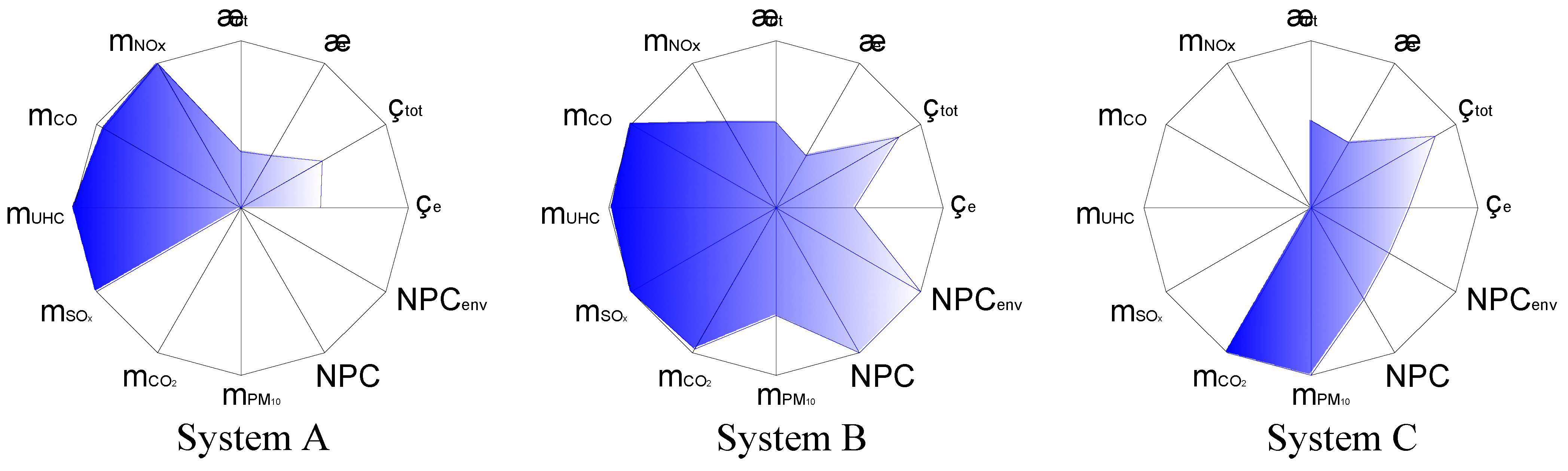
4.2. Graphical Presentation of the Results

It is common practice in multi-criteria analyses to present the results on an “amoeba” plot. The plots obtained with the values of the indicators (Table 10) appear in Figure 2.
Figure 2. Amoeba plots of indicators for the alternative systems.
Entropy 12 01006 g002
The amoeba plots have two disadvantages: (i) the surface area depends on the order in which the indicators are placed, and (ii) it is not easy to calculate the surface area. Thus, the viewer obtains a general impression but not concrete values. In order to overcome these disadvantages, a presentation by means of sectors in a circle is proposed here, as it appears in Figure 3: the radius of the sector corresponding to the normalized indicator I ¯ i j is equal to the value of I ¯ i j . The angles between the indicators are equal to each other, if the relative weights are the same. The surface area of the plot is equal to the summation of the surface areas of the sectors:
A = i j A i j = π N I i j I ¯ i j 2
where NI is the total number of indicators. Furthermore, since the maximum surface area of the plot is equal to the surface area of the circle with radius equal to 1, i.e. A max = π , a normalized value of A can be defined:
A ¯ = A A max = 1 N I i j I ¯ i j 2
The results for the three systems are as follows:
A ¯ A = 0.3338    A ¯ B = 0.5027    A ¯ C = 0.3056
Sectorial plots can be drawn also with the sub-indices, as shown in Figure 4.
Figure 3. Sectorial plots of indicators for the alternative systems.
Entropy 12 01006 g003
Figure 4. Sectorial plots of sub-indices for the alternative systems.
Entropy 12 01006 g004
In this case, the following equations are applicable for each system:
A S = j A j = π N j j I ¯ S j 2
A ¯ S = A S A max = 1 N j j I ¯ S j 2
The results for the particular systems are the following:
A ¯ S A = 0.2068    A ¯ S B = 0.6834    A ¯ S C = 0.2739

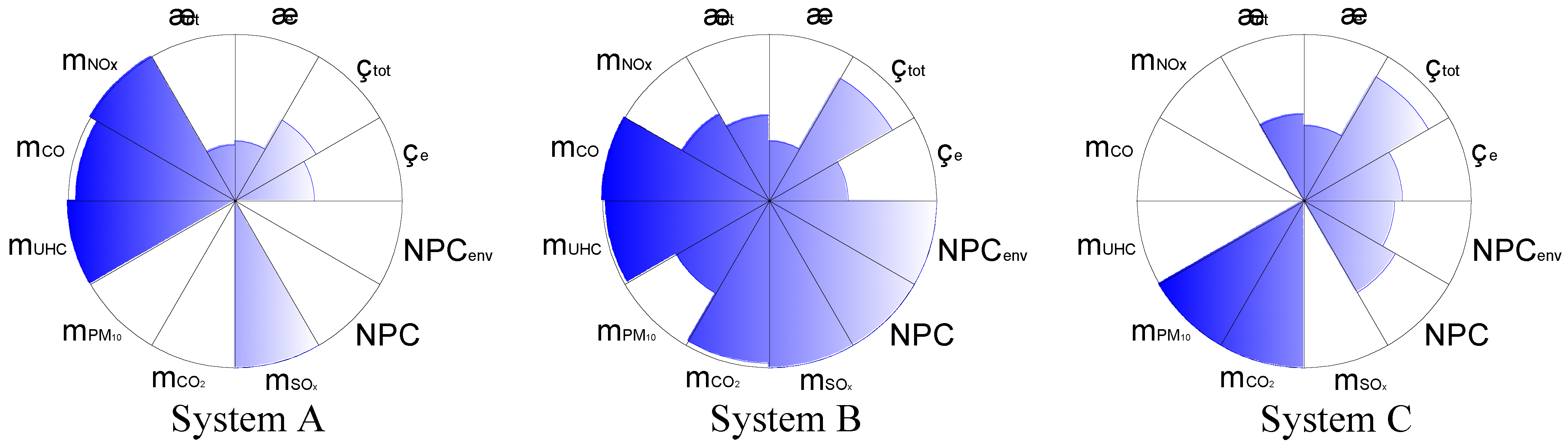
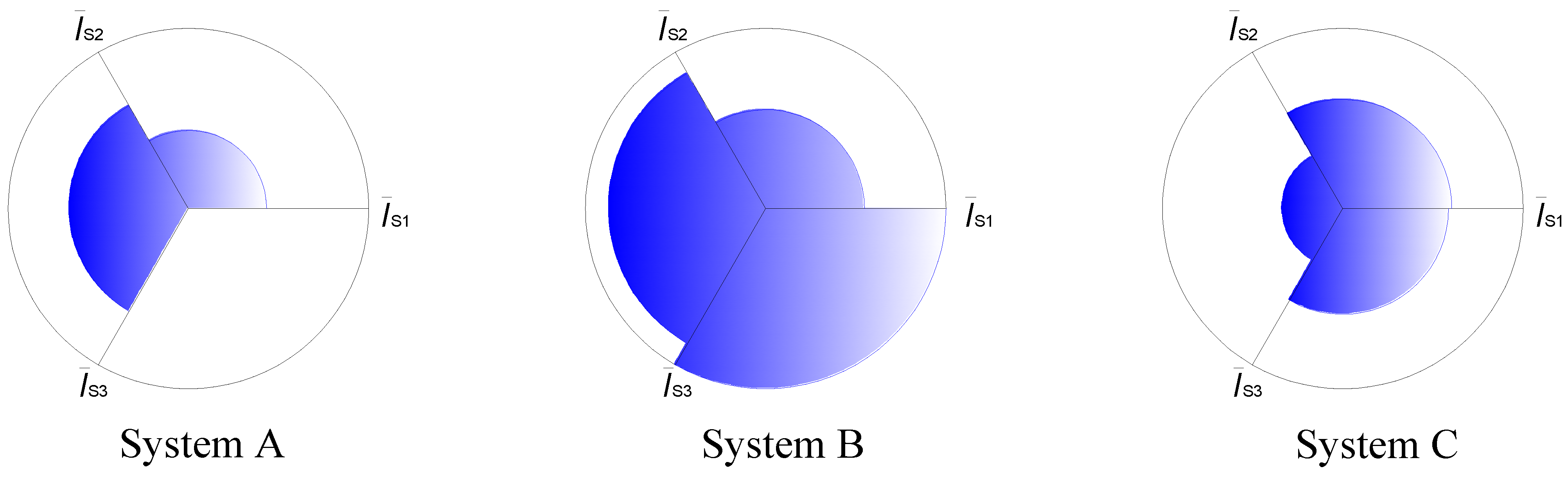
4.3. Comments on the Results

The results of Subsections 4.1 and Subsections 4.2 lead to the following comments. With pure thermodynamic criteria (efficiencies), the best option is the dual fuel unit combined with a boiler for supplementary thermal energy, while the gas turbine cogeneration system comes second. This is due to the high electric efficiency of the dual fuel engine, which gives a high exergetic efficiency for this system.
From the environmental point of view, the best option is the gas turbine system and the worst option is the system with the duel fuel engine, because of relatively high NOx, CO and UHC emissions (according to the source of related information used in this work).
From the economic point of view, either with or without environmental externalities, the best option is the gas turbine cogeneration system, while the worst option is the separate production of electricity and heat.
If the indicators are taken into consideration not in groups but individually, then the best option is still the gas turbine system, but the worst one is the system with the duel fuel engine (Figure 2 and Figure 3, and values of A ¯ A , A ¯ B , A ¯ C ). The same order of preference is indicated also with the arithmetic average of the twelve indicators (Table 10). This is due to the fact that the environmental indicators have a stronger impact due not only to their values, but also to their number: they are six, while the thermodynamic indicators are four and the economic indicators are only two.
The composite sustainability index gives the same order of preference as the economic indicators (Table 11 and Figure 4).

4. Conclusions and Recommendations

With the multi-criteria evaluation procedure presented in the preceding sections, the performance of an energy conversion system from various points of view can be assessed and the alternatives available for covering energy needs can be compared with each other from various points of view. It is advisable that such a procedure is applied to complement the usual energetic, exergetic, economic or thermoeconomic analysis. The sectorial plot is introduced here as a clearer (as compared to the usual amoeba plot) picture of a multi-criteria assessment.
It is important to note that the order of preference among alternatives is affected by grouping of the indicators: the more indicators are placed in a group, the weaker their impact on the composite sustainability index.
In the procedure applied in this work, fuel is the only resource taken into consideration and this is done implicitly through the efficiencies. It is useful to supplement the evaluation procedure with indicators derived with a life-cycle approach (e.g., eco-indicators).
Even though the social aspects have been mentioned in the preceding, lack of sufficient data did not allow for the inclusion of social indicators in this work. It is desirable to supplement with the required knowledge and include such an important aspect in the evaluation procedure with future research work.

References

  1. WCED. Our Common Future. In Report of the UN World Commission on Environment and Development, Gro Harlem Brundtland, Chair; Oxford University Press: Oxford, UK, 1987. [Google Scholar]
  2. Lior, N. About sustainability metrics for energy development. In Proceedings of the 6th Biennial International Workshop “Advances in Energy Studies”, Graz, Austria, 29 June–2 July 2008; pp. 390–401.
  3. Keramioti, D.E. Performance Evaluation Of Energy Systems With Sustainability Considerations. Diploma Thesis, National Technical University of Athens, School of Naval Architecture and Marine Engineering, Athens, Greece, October 2009. [Google Scholar]
  4. Afgan, N.H.; Carvalho, M.G. Sustainable Assessment Method for Energy Systems: Indicators, Criteria and Decision Making Procedure; Kluwer Academic Publishers: Boston, MA, USA, 2000. [Google Scholar]
  5. Tonon, S.; Brown, M.T.; Luchi, F.; Mirandola, A.; Stoppato, A.; Ulgiati, S. An integrated assessment of energy conversion processes by means of thermodynamic, economic and environmental parameters. Energy 2006, 31, 149–163. [Google Scholar] [CrossRef]
  6. Krajnc, D; Glavič, P. How to compare companies on relevant dimensions of sustainability. Ecol. Econ. 2005, 55, 551–563. [Google Scholar] [CrossRef]
  7. Afgan, N.H.; Carvalho, M.G. Sustainability assessment of hydrogen energy systems. Int. J. Hydrogen Energy 2004, 29, 1327–1342. [Google Scholar] [CrossRef]
  8. Valero, A.; Lozano, M.A.; Serra, L; Tsatsaronis, G.; Pisa, J; Frangopoulos, C; von Spakovsky, M.R. CGAM Problem: Definition and conventional solution. Energy 1994, 19, 279–286. [Google Scholar] [CrossRef]
  9. Frangopoulos, C.A. Application of the Thermoeconomic Functional Approach to the CGAM Problem. Energy 1994, 19, 323–342. [Google Scholar] [CrossRef]
  10. COGEN Europe. EDUCOGEN—The European Educational Tool on Cogeneration, 2nd Edition. ed; The European Association for the Promotion of Cogeneration: Brussels, Belgium, 2001; Available online: http://www.cogen.org/projects/educogen.htm/.
  11. Dorai, V.S.; Frangopoulos, C.A. Estimation of Environmental Externalities and their Effect on the Optimization of a Cogeneration system. In 21st International Conference on Efficiency, Cost, Optimization, Simulation and Environmental Impact of Energy Systems, ECOS 2008, Kraków, Poland, 24–27 June 2008; pp. 1419–1428.

