1. Introduction
Industrial Ecology (IE) offers promising opportunities for attaining sustainable industrial development. IE essentially aims at achieving a more rational and balanced industrial organization, trying to imitate the structure and operation of natural ecosystems. Like natural organisms, industrial ecosystems consume material, energy and water flows, transforming them into products and wastes. However there is one important difference among the two: the wastes produced by natural organisms are used as feedstock for other natural systems. As a result of this cyclic process, the net production of wastes produced in nature is zero. Wastes are always a consequence of lack of knowledge. The challenge of industrial systems is thus to identify opportunities for waste reduction by imitating nature (industrial biocenosis). Instead of the
Zoo paradigm in which any industry must be fed and cleaned up separately, the
Savannah paradigm must prevail. In the latter, every facility feeds products/wastes from someone else and ultimately the natural surroundings act as another active member of the industrial community. In Industrial Ecology, the conventional linear productivity chain approach is shifted into a materials cycle approach [
1]. Unfortunately, the dominant industrial conception has been so far that of the Zoo paradigm, constituting a fundamental factor in the current environmental crisis.
Industrial Ecology principles are materialized through the establishment of eco-industrial parks. These are defined as “a community of businesses that cooperate with each other and with the local community to efficiently share resources (information, materials, water, energy, infrastructure and natural habitat), leading to economic gains, gains in environmental quality, and equitable enhancement of human resources for the Business and local community” [
2]
Frosch and Gallopoulos [
3], Dunn and Steinmann [
4], Chertow [
5,
6] or Gibbs
et al. [
7] analyze in detail the strengths and barriers of IE. Particularly, the latter two authors make a critical evaluation of eco-industrial parks in development. Some of the economic, environmental and social advantages listed in the literature are the following:
The input costs of raw materials are reduced as waste products from one industry are provided as inputs for another.
Wastes are converted into products with an associated economic value.
The waste streams are reduced and hence the disposal costs.
Enhancement of long-term resource security by increasing the availability of critical resources such as water, energy or particular raw materials through contracts.
Creation of a larger and more varied economic base.
Potential for job creation from the formation of niche species firms.
Although theoretically IE represents a win-win situation, the associated benefits are difficult to evaluate and have seldom been carefully measured. A critical barrier commonly encountered when promoting eco-industrial parks is in encouraging companies for pursuing industrial symbiosis. The most obvious motivations are conventional business reasons; for example, resource sharing can reduce costs and/or increase revenues [
5]. But companies will unlikely act with mere qualitative statements no matter how promising they are. Companies need numbers and these numbers should be as objective and accurate as possible.
The integration of industrial systems with mutual exchanges of resources, products and wastes implies energy savings. And the most objective way to analyze the magnitude of those savings is through the laws of Thermodynamics. As stated before, in all industrial processes, energy resources are consumed and non energetic raw materials are transformed. In this context, exergy rather than energy is the unit of measure to be used. In every material and energy transformation, neither matter, nor energy disappear, it is always exergy what is lost. Each step in the manufacturing process involves the generation of irreversibilities and hence of exergy losses (often misinterpreted as energy losses). The most important contribution of the exergy concept is in its ability to objectify all the physical manifestations in energy units, independently of their economic value. Any product, natural or artificial resource, productive process or polluting emission can be valued from an exergy point of view with a single unit of measure.
A number of authors such as Ayres and Ayres [
8] have long been stating that the exergy analysis can help to quantify the benefits of Industrial Ecology. In particular, Connelly and Koshland [
9] discussed the ties between exergy and industrial ecology and proposed exergy-based definitions and methods for addressing resource depletion. Finnveden and Östlund [
10], Cornelissen and Hirs [
11] and Dewulf and Langenhove [
12,
13] applied the exergy analysis to the Life Cycle Assessment (LCA) methodology, which should account for the depletion of natural resources and the associated environmental impacts.
Unfortunately, exergy analysis is necessary but not sufficient to determine the origin of losses and the potential for energy saving. Conventional Thermodynamics states that the exergy balance accounts for the degradation of the exergy. The incoming exergy will be always greater than the outgoing one:
This expression only points out the existence of irreversibilities within the process. However Thermoeconomics (TE), term coined by Tribus and Evans [
14], takes a step further, including in this equation the concept of purpose by means of the definition of efficiency. This is to say that there is an implicit classification of the flows crossing the boundary of the system: the production objective,
P, the resources required to carry out the production,
F, and those that are residuals or wastes,
R. We cannot just associate the resources with input flows, nor the products with output flows. We need to have a clear idea of what we want to produce before defining the efficiency. This information is not implicit in the Second Law and is the most important conceptual leap separating and at the same time unifying Physics with Economics. This way, the exergy balance now becomes:
where
I represents the irreversibilities of the process. All resources have an “economic” cost: the more irreversible a process is the more resources and energy are consumed (higher exergy cost). The concept of exergy cost is still within Thermodynamics, but it already shares many of the cost accounting methodologies borrowed from Economics. It is clearly a conceptual link between these two disciplines. Thus the isomorphism between exergy cost and economic cost lets us straightforwardly convert thermodynamic costs into thermoeconomic costs, by simply adding the prices of resources, installation and maintenance costs. In fact, this methodology is isomorphous with the Input-Output analysis [
15], with the difference that Thermoeconomics uses Second Law to cost assessment. This is the only way that we can provide physical roots to the accounting techniques. The cost formation process sheds light on new paths for economic, scientific, technological and, perhaps, philosophical research. Thermoeconomics becomes a crystal clear and unique way to connect the universal measure of physical loss,
i.e., irreversibility with the loss of resources at the overall system level and then to Economics. The “exergy cost” concept was proposed by Valero
et al. [
16]. Almost simultaneously Szargut and Morris [
17] proposed the “cumulative exergy consumption” theory. Both concepts represent in fact embodied exergy.
Thermoeconomics has been largely used for the diagnosis of single production plants, allowing the identification of inefficiencies and the potential for energy savings [
18]. Now, it is the time to open the approach to industrial networks under the industrial ecology paradigm. The versatility of TE allows its application to complex systems, providing a systematic and general approach for the analysis of waste flow integration.
On the other side, Input-Output analysis (IO) has been used to address environmental issues related to Industrial Ecology [
19] and Environmental Life Cycle Assessment [
20]. However, it IO has been traditionally used with different quantity units for accounting for all energy and material fluxes coming into play, what complicates extremely the analysis. Similarly, if monetary units are used to assign costs, it may introduce arbitrariness to the analysis. As it has been argued before, exergy is a suitable physical unit to which costs should be allocated. To this same conclusion have come Hau and Bakshi [
21], who applied exergy and cumulative exergy consumption, to Input-Output analysis in a sample of industrial and ecological systems.
In short, the application of exergy to IO analysis based on Thermoeconomics can help to rationalize the general problem of energy saving achieved through waste integration. Moreover, it is able to objectively assess the final costs of the products interchanged in eco-industrial parks, providing a decision tool for companies.
In the following sections, a description of the fundamentals of Thermoeconomics applied to an Industrial Ecology is developed, and an example is carried out.
2. The Thermoeconomic Model
For the thermoeconomic characterization of any energy system, a thermoeconomic model is firstly required. In the following sections, the basic ingredients of the thermoeconomic model are briefly described.
2.1. Physical Structure
Energy systems represent complex networks of mass and energy flows. The level of aggregation of the system depends on the type of analysis carried out. The total system is composed of a collection of subsystems. Each subsystem can be a part of a physical device, the device itself or a group of devices, representing the thermodynamic process.
A suitable data structure representation of an energy system for a specific level of aggregation is made by means of a directed graph, consisting of a set of graph nodes representing the system components, and a set of graph edges, where each element connects two components of the system and shows the interchanged mass or energy flows.
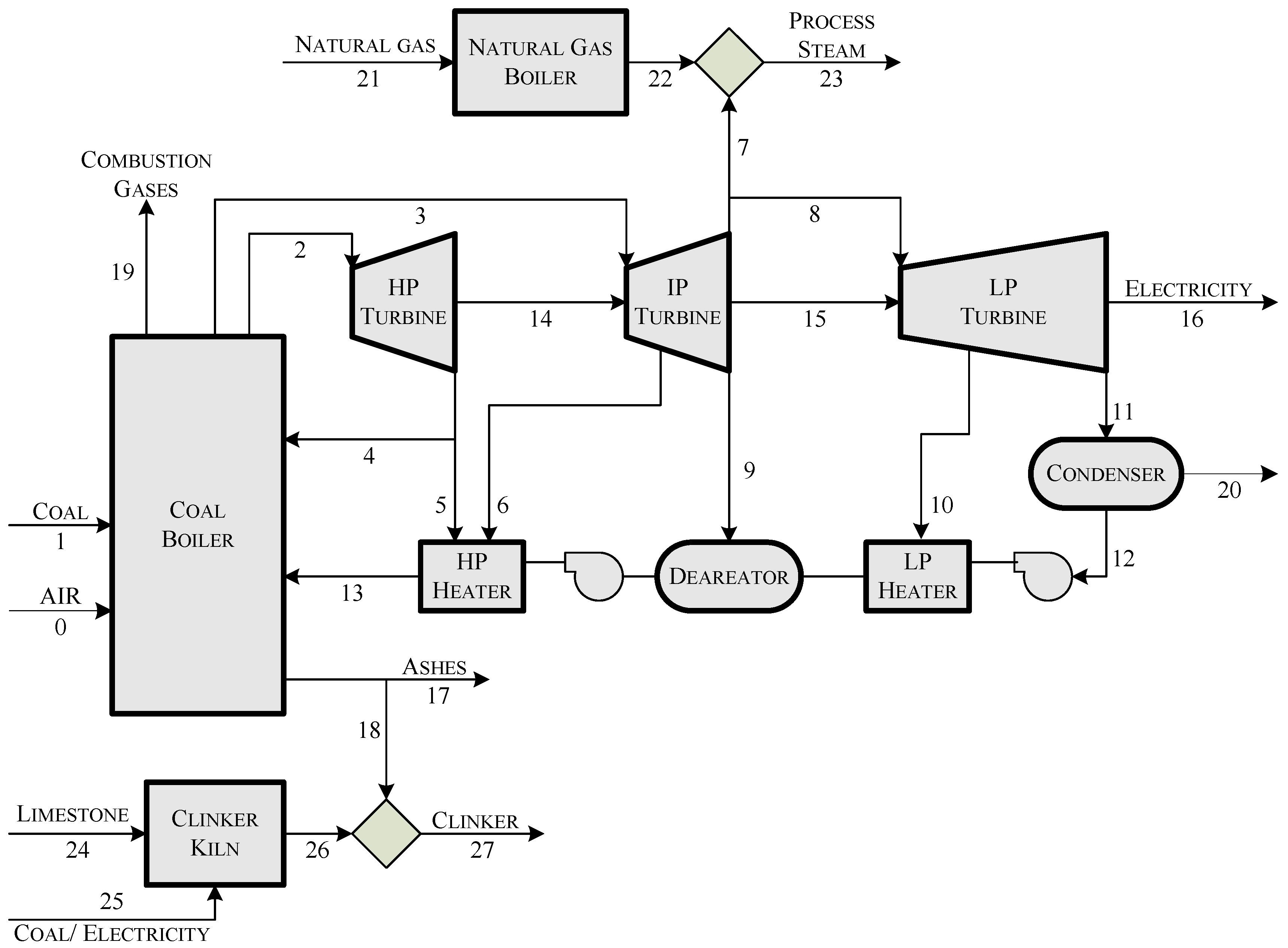
Figure 1 shows an example of the physical structure of an eco-industrial park which integrates a power plant, a steam generator and a cement factory. In the figure, the boxes represent the components and the arrows the flows of the system.
Figure 1.
Physical structure of an eco-industrial park, integrating a power plant, a steam generator and a cement factory.
Figure 1.
Physical structure of an eco-industrial park, integrating a power plant, a steam generator and a cement factory.
2.2. Thermodynamic Model
The thermodynamic model (TDM) of the plant is described through a set of equations, (including the mass, energy and entropy balances). They allow every mass flow stream and every heat and work interactions involved in the physical structure of the plant to be determined from a set of input variables, defining a thermodynamic state of the plant. Exergy is used as the measure of the usefulness of the energy carried by each flow defined in the physical structure.
2.3. Fuel and Product
Each component or process of the system has a productive purpose. It is established by means of the definition of its efficiency:
Efficiency measures the quality of a process. This is to say, there is an implicit classification of the flows crossing the boundary of the system, the flows that are the production objective, and those that are the resources required to carry out the production. Since the exergy of resources is greater than that of the products, this efficiency is always positive and less than one.
For each process or component of the system, it is necessary to identify the flow streams that constitute its
product streams, and the flow streams used to obtain them, called
fuel streams. Accordingly, it can be said that the
fuel is the amount of exergy provided by the resources streams, and the
product is the exergy provided by the product streams.
Table 2, shows the fuel–product definition for the components of the system depicted in
Figure 1.
2.4. Waste and By-Products
In any productive process, along with the primary products, there are unintended remaining output flows of matter or energy called
residuals or
wastes. Waste refers to those outputs which are disposed of. They could also be partially used in further processes,
i.e.,
recycled. Therefore, besides the
productive components, there are components whose objective is to dissipate residual flows. Our technical limitations make these components to be a need, since we are not able to recover all the exergy of outputs and they become wastes. The combustion process is an example of this fact. It has a low efficiency conversion, and furthermore it produces low thermal exergy residual gases which cannot be recovered and must be disposed of into the environment. Moreover, if we want to eliminate them, additional resources are required, using processes to cooling, expanding, dispersing or capturing them. The efficiency of a dissipative unit measures the amount of resources required per unit of exergy reduced in the waste flow:
Since the resources required have no relationship with the decreased exergy of waste, this efficiency is always positive and does not have an upper limit of one.
Thermoeconomics has been mainly focused on production and dissipative processes, but there is also another type of system outputs which belongs neither to primary products nor to waste, and they are called by-products.
According to Nakamura and Kondo [
22] we incorporate the following definitions of by-products:
An output from a given production process is a competitive by-product, when it is not a primary product of the process, but technically related to its production, and happens to be the primary product of another production process.
An output from a given production process is a non-competitive by-product, when it is not a primary product, but related to its production and there is not another production process where it is primary produced.
Competitive by-products are part of the output of productive or dissipative units that could be used total or partially as alternative products in other processes. An example of this kind of by-product is the steam produced in a power plant and further used as process steam in a chemical plant, which also produces steam in a natural gas boiler.
Non-competitive by-products are closely related to waste recycling. Ash generated by an incinerating process or coal burned in power plants is a typical example of this type of by-product associated with waste treatment processes. Ash can be used as a raw-material for cement production within a limited range as a substitute for clinker.
The output flows that belong neither to products nor to waste are emissions, examples of which are CO2, NOx and SOx in the exhaust gases of combustion processes.
2.5. Productive Structure
The productive structure [
23] is the representation of the production process of an energy system. The inputs of each process are the resources or fuels and the outputs are their products. The utility of the obtained products can be of different nature: as fuels for other components, as part of the primary product, as by-products or as wastes that must be eliminated in dissipative or waste treatment components. Reciprocally the fuel of a component comes from external resources or from the products of another component. The definition of the
productive structure depends on the definition of the efficiency of the individual components of the system for a given aggregation level. The fuel and product of a component do not necessarily correspond with the input and output of the physical components. For example in a power plant turbine, the product is the mechanical energy produced, meanwhile the fuel is the difference between the exergy of the input and output steam flows. Furthermore, the components of the productive structure could be different from those of the physical structure. This way, some physical components could be disaggregated for a better analysis of its products and wastes and vice versa, they could be aggregated to simplify the model without loss of information.
For the description of the
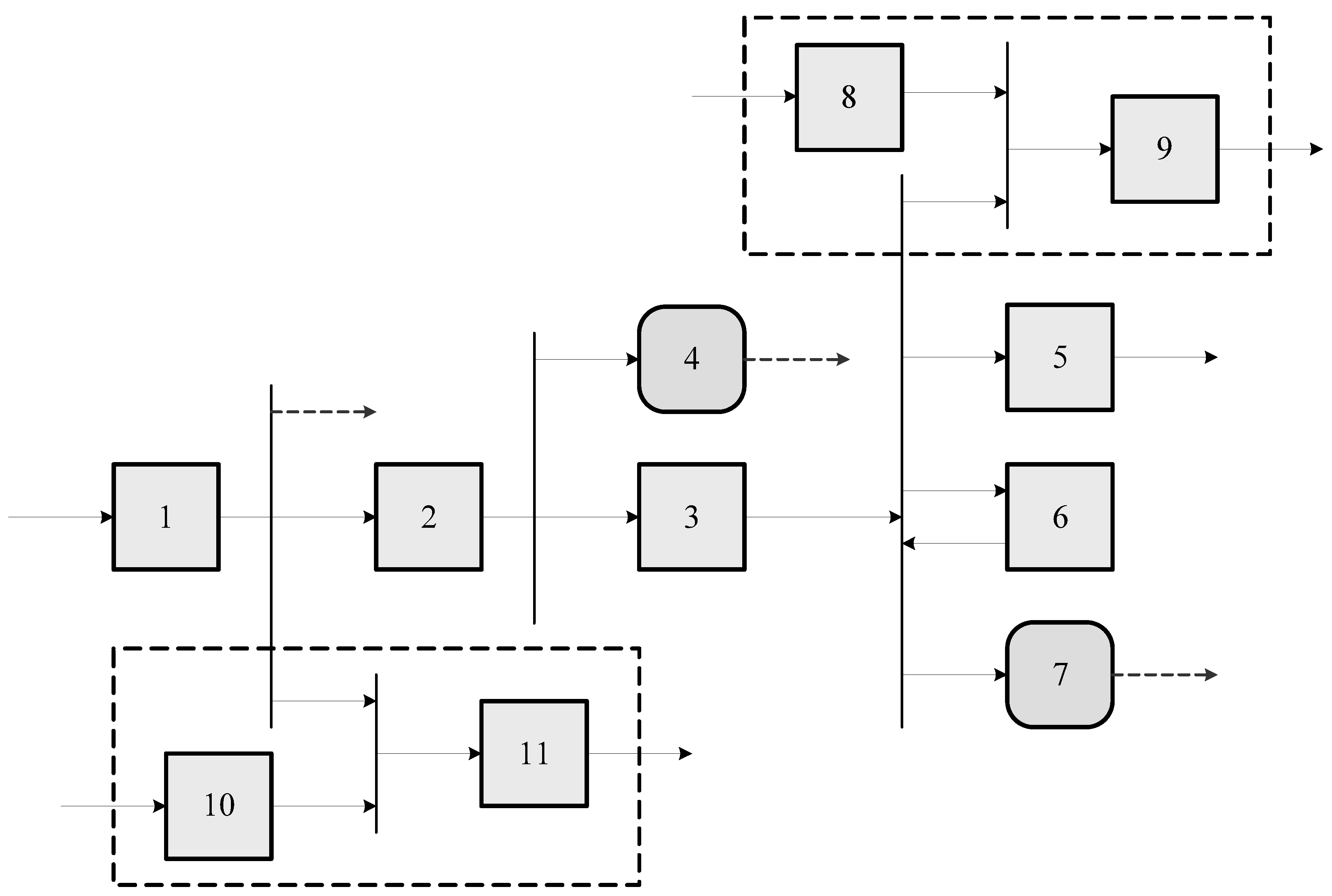
productive structure we must identify, for every component, one or several fuel and product streams. From the fuel-product definition it is possible to build a productive diagram, as the one shown in
Figure 2.
The productive structure is the key point to understand the cost formation process of products, by-products and wastes.
2.6. External Resources Assessment
The definition of the thermoeconomic model requires also every external resource inputs to the system to be valued. The ways these external resources are valued will determine the type of cost obtained. If the resources are accounted in terms of exergy, the results obtained are expressed as exergy costs (kW). Alternatively, if the cumulative exergy for the complete life cycle of the resources is used, then exergy life costs (kW) will be obtained.
Figure 2.
Productive Structure of the integrated plant.
Figure 2.
Productive Structure of the integrated plant.
Thermoeconomics can also use economic valuation of the external resources costs. In this case the resulting cost is evaluated in monetary units per unit of time (€/h) and is called
exergoeconomic cost. The latter includes:
The investment and operational cost of the equipment (€/h), defined as a function of a list of parameters, including size, materials, operating range, working hours per year, inflation rates, installation and maintenance cost, as well as other factors, see [
24].
The market prices of the fuels (€/kWh), natural gas, coal and other external resources.
The cost (€/h) of the resources required for the disposal of the wastes, or abatement costs.
3. The Fuel-Product-Residuals Model
The first step for the identification of the cost formation process of products and wastes consists of building a productive scheme that explains the resources distribution throughout the plant. This approach, which is closely related to
Input-Output analysis, is essential in order to analyze the potential improving of recycling. An equivalent micro-economic model based on the Second Law of Thermodynamics, can be applied to energy systems. This model can be represented by means of an input-output table (see
Table 1). The rows represent the destination of the production of each component: as fuel of other components, as disposable waste, or as a primary product of the system. The first row represents the external resources entering the system. Meanwhile, the columns represent the source of the fuel of each component: either coming from the production of other components or as resources coming from outside the boundaries of the system. An algorithm to obtain the fuel-product table from the physical and productive structure is described in [
25].
Table 4 shows the Fuel-Product tables of the integrated system used in our case study.
Table 1.
Generic FP Table.
Table 1.
Generic FP Table.
| | F | … | F | … | F | | |
| | … | | … | | | |
| P | | … | | … | | | |
| … | … | … | … | … | … | … | … |
| P | | … | | … | | | |
| … | … | … | … | … | … | … | … |
| P | | … | | … | | | |
According to this representation, the production of a productive component is used as fuel of other components or as a primary product of the system. Mathematically, this could be expressed as the sum of the element of each fuel-product table row:
In the above expression, if the component 0 is considered to be the system environment, then
represents the production of the
i-th component that leaves the system as a primary product. In case of waste treatment units
represents the disposable, or not recycled, waste.
On the other hand, the resources consumed by each component are the sum of the elements of each fuel-product table column:
where
represents the external resources used in the
i-th component.
The exergy balance, Equation (
1), is the point in understanding the difference between the Input-Output quantity model and the Thermoeconomic approach. The only numeraire (kg, m
, kJ,…) defining F, P and R that satisfies the Second Law Analysis is exergy. The right hand side of this equation is the measure of the process irreversibility. Since all elements in the fuel-product table are measured in the same quantity exergy, it is possible to add not only the rows (products) but also columns (fuels) for each component and compare them. The comparison between fuels and products provides a universal measure of the quality of a process.
Equations (
2) and (
3) can be compactly summarized in matrix notation as:
where
is a square matrix
which represents the internal elements of the Fuel-Product table.
and
are column vectors
that represent the fuel and product of each component.
and
are column vectors
that represent the exergy of primary output and the waste generated for each component.
is a
column vector that contains the exergy of the external resources entering each component. We use
to represent a column vector of 1’s (with the appropriate dimension–here
n is the number of components). An important observation is that post-multiplication of a matrix by
creates a column vector whose elements are the row sums of the matrix. Similarly
is a row vector of 1’s and premultiplication of a matrix by
creates a row vector whose elements are the column sums of the matrix. We will use these “summation” vectors along the paper.
Let define the
exergy distribution ratios as
as the part of the production of the
component becoming fuel of the
component. If we denote by
the square matrix
which contains the exergy distribution ratios of the system, then it verifies:
we use
to represent a diagonal matrix, whose elements are a vector
.
5. Application to a Plant Integration Analysis
The aim of this section is the application of the methodology previously developed in a case study. Three installations have been considered: a coal-fired power plant, a cement plant and a gas-fired boiler producing steam. Besides, two integrations are analyzed: use of steam bleeding instead of steam produced by the gas-fired boiler, and use of part of fly ashes for substituting clinker within the cement industry.
A simplified physical structure of the system has been depicted in
Figure 1. The main facility is a power plant producing 350 MW at design conditions. In addition to superheated and reheated steam, the coal-fired boiler produces ash and a flow of flue gases. The steam cycle is composed of high pressure, medium pressure and low pressure steam turbines. Steam leaving the last turbine is condensed and then compressed and heated by both low pressure and high pressure heaters and a deaerator (consuming bleeding steam) prior to enter the boiler to close the cycle. Part of the steam leaving the medium pressure steam turbine can be diverted from the steam cycle and used in industrial processes.
The cement plant considered has a capacity of 650,000 ton/year operating 8,000 hours/year. The cement manufacturing process can be divided into two parts: clinker production taking place in a kiln and grinding and mixing of this clinker with other constituents. The clinker production process begins with the calcination of limestone (mainly CaCO3) at about 900C to form calcium oxide (CaO, lime). This is followed by the clinkering process in which the calcium oxide reacts at high temperature (typically 1400–1500C) with silica, alumina, and ferrous oxide to form clinker. The clinker is then milled with gypsum and other additives to produce cement. It should be noted that it is possible to replace part of the clinker by fly ash.
Finally, the gas-fired boiler produces a flow of 10 kg/s of steam at 8.5 bar and 310C. These intensive properties have been fixed to coincide with those of steam leaving the medium pressure turbine of the power plant.
In order to perform the thermoeconomic analysis, a productive structure comprising power plant, cement kiln and gas-fired boiler has been defined and represented in
Figure 2. Since this structure focuses on the purpose of the sub-systems, it contains not only actual devices appearing in the physical structure but mainly groups of them as well as fictitious components for joining and diverting flows. Components of the productive structure as well as their efficiency definition are shown in
Table 2.
The coal boiler is disaggregated into three components: Component #1 is a fictitious device which removes the ashes from the coal, and part of the ashes are recycled and used in the cement plant. Component #2 is the combustion chamber that transforms the exergy of coal without ashes into a flow of heat at adiabatic flame temperature, whose exergy is denoted by . It also produces a flow of flue gases going to stack (#4). Component #3 represents the boiler heat exchange and uses the heat flow to produce steam that is used in further processes as well as heat released in the condenser (#7).
Component #5 aggregates the three stages of the turbine and transforms steam into electricity. Component #6 aggregates the feedwater heaters. It uses part of bleeding steam to produce hot water returning to the boiler.
Component #9 is a junction connecting steam produced by the natural-gas boiler (#8) with steam bleed from the steam cycle in order to produce a flow to be used in an external process. Besides, component #11 is another junction which connects clinker from the kiln (#10) with ash imported from the power plant.
Table 2.
Productive Structure Definition.
Table 2.
Productive Structure Definition.
| Nr | Component | Fuel | Product |
|---|
| 1 | Ash separator | | |
| 2 | Burner | | |
| 3 | Boiler | | |
| 4 | Stack | | |
| 5 | Steam turbines | | |
| 6 | Feedwater heaters | | |
| 7 | Condenser | | |
| 8 | Natural-gas boiler | | |
| 9 | Steam mixer | | |
| 10 | Cement kiln | | |
| 11 | Clinker mixer | | |
Exergy flows of the power plant have been adapted from [
27] and correspond to an actual operation point of the plant. An exception is the ash flow which has been obtained by considering a coal heating value of 16,912 kJ/kg, a coal ash content of 23.16% and an ash composition of 49% SiO
2, 26% Al
2O
3, 15% CaO and 10% Fe
2O
3, which results in an exergy value of 454.0 kJ/kg). Values of exergy related to gas-fired boiler have been calculated by considering an energy efficiency of 0.9 (exergy efficiency is lower). In the case of the cement kiln, it has been considered that each kg of clinker needs 1.54 kg of raw material (mainly limestone) and 4,195 kJ of fuel, including a small part of electricity [
28]. Specific exergies of the raw material and clinker are 220 kJ/kg and 1,240 kJ/kg respectively, see reference [
29].
In the integrated plant, steam flow produced by the natural-gas boiler is completely substituted by a similar flow bleed from the steam cycle, while the power plant electricity production is kept constant. Accordingly, the amount of coal burned in the power plant increases. Besides, 10% of the mass flow rate of clinker produced in the kiln is substituted by fly ashes imported from the power plant, which has two effects. First, the amount of resources consumed by the kiln is reduced, and, second, exergy flow of the cement also varies because each kg of ash replaces one kg of clinker while the specific exergy of the former is smaller than the specific exergy of the latter.
Table 3.
Waste cost distribution ratios matrix.
Table 3.
Waste cost distribution ratios matrix.
| | 1 | 2 | 3 | 4 | 5 | 6 | 7 | 8 | 9 | 10 | 11 |
| 1 | 1.0 | 0 | 0 | 0 | 0 | 0 | 0 | 0 | 0 | 0 | 0 |
| 4 | 1.0 | 0 | 0 | 0 | 0 | 0 | 0 | 0 | 0 | 0 | 0 |
| 7 | 0 | 0 | 0.58 | 0 | 0.11 | 0.31 | 0 | 0 | 0 | 0 | 0 |
The last point to be considered is to define the distribution of costs associated with wastes. It is done by means of the waste cost cost distribution ratios matrix
. Their values for the case study system are shown in
table 3. There are three components producing wastes: ash separator (#1) producing ash, stack (#4) producing flue gases and condenser (#7) producing waste heat. Both costs associated to ash and flue gases are charged to the ash separator. The cost of waste heat from the condenser is shared proportionally to the entropy generation in the different elements of the steam cycle. Abatement costs for ashes landfilling, combustion gases and cooling system are not considered, but it could be included here, is a more detailed analysis.
6. Results Analysis
Prior to present the results obtained with the application of the methodology to the case study, it is useful to consider what is needed in the evaluation of the integration of several subsystems. Obviously, the main question is which are the savings achieved. However it is interesting to go beyond in order to understand where these savings come from and how they are formed. This can be done by applying thermoeconomic analysis.
The fuel-product tables for the non integrated and integrated system are shown in
Table 4. In the first case (a), the power plant, cement plant and natural gas boiler work independently, producing respectively electricity, clinker and steam. In the second case (b) the plants are integrated. Each row of the tables represents how the product of a component is distributed among the other components, how it forms a final product or how it becomes a waste. For example, in
Table 4(a), burner (#2) produces 740.8 MW of hot flue gases for the steam boiler (#3) and 37.7 MW are dissipated in the stack (#4). Besides, in each column, the origin of fuel of each component can be seen, for example, the fuel of the turbines (#5) comes from the boiler (#3) and from the feedwater heaters (#6).
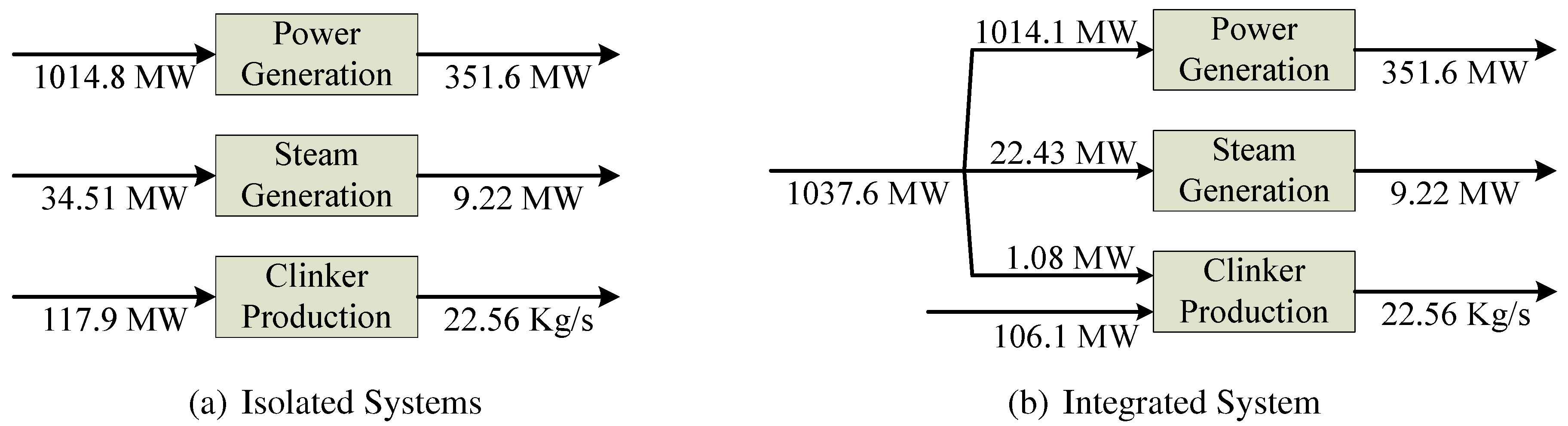
Figure 3 resumes the exergy savings achieved by the integration. In the original situation, the total fuel consumption is 1167.2 MW, meanwhile with the integration it decreases down to 1143.7 MW. Therefore, the total fuel saving is equal to 23.5 MW (2%), which may seem small compared to the global consumption, but corresponds to more than €3.5 million/year. The exergy saving for process steam is 12.08 MW (34%), and the exergy saving in clinker production is 11.84 MW (9%).
Table 4.
Fuel–Product Table in MW for isolated (a) and integrated (b) system.
Table 4.
Fuel–Product Table in MW for isolated (a) and integrated (b) system.
| (a) Isolated system |
| | F | F | F | F | F | F | F | F | F | F | F | | | Total |
| 1014.8 | 0 | 0 | 0 | 0 | 0 | 0 | 34.51 | 0 | 117.9 | 0 | 0 | 0 | 1167.2 |
| P | 0 | 1008.5 | 0 | 0 | 0 | 0 | 0 | 0 | 0 | 0 | 0 | 6.31 | 0 | 1014.8 |
| P | 0 | 0 | 740.8 | 37.7 | 0 | 0 | 0 | 0 | 0 | 0 | 0 | 0 | 0 | 778.5 |
| P | 0 | 0 | 0 | 0 | 347.8 | 97.92 | 52.92 | 0 | 0 | 0 | 0 | 0 | 0 | 498.6 |
| P | 0 | 0 | 0 | 0 | 0 | 0 | 0 | 0 | 0 | 0 | 0 | 37.73 | 0 | 37.73 |
| P | 0 | 0 | 0 | 0 | 0 | 0 | 0 | 0 | 0 | 0 | 0 | 0 | 351.6 | 351.6 |
| P | 0 | 0 | 0 | 0 | 62.28 | 17.54 | 9.48 | 0 | 0 | 0 | 0 | 0 | 0 | 89.29 |
| P | 0 | 0 | 0 | 0 | 0 | 0 | 0 | 0 | 0 | 0 | 0 | 49.01 | 0 | 49.01 |
| P | 0 | 0 | 0 | 0 | 0 | 0 | 0 | 0 | 9.22 | 0 | 0 | 0 | 0 | 9.22 |
| P | 0 | 0 | 0 | 0 | 0 | 0 | 0 | 0 | 0 | 0 | 0 | 0 | 9.22 | 9.22 |
| P | 0 | 0 | 0 | 0 | 0 | 0 | 0 | 0 | 0 | 0 | 27.99 | 0 | 0 | 27.99 |
| P | 0 | 0 | 0 | 0 | 0 | 0 | 0 | 0 | 0 | 0 | 0 | 0 | 27.99 | 27.99 |
| Total | 1014.8 | 1008.5 | 740.8 | 37.73 | 410.0 | 115.5 | 62.40 | 34.51 | 9.22 | 117.9 | 27.99 | 93.05 | 388.21 | |
| (b) Integrated System |
| | F | F | F | F | F | F | F | F | F | F | F | | | Total |
| 1037.6 | 0 | 0 | 0 | 0 | 0 | 0 | 0 | 0 | 106.1 | 0 | 0 | 0 | 1143.8 |
| P | 0 | 1031.2 | 0 | 0 | 0 | 0 | 0 | 0 | 0 | 0 | 1.03 | 5.43 | 0 | 1037.6 |
| P | 0 | 0 | 757.5 | 38.58 | 0 | 0 | 0 | 0 | 0 | 0 | 0 | 0 | 0 | 796.0 |
| P | 0 | 0 | 0 | 0 | 347.8 | 97.92 | 52.92 | 7.82 | 0 | 0 | 0 | 0 | 0 | 506.4 |
| P | 0 | 0 | 0 | 0 | 0 | 0 | 0 | 0 | 0 | 0 | 0 | 38.58 | 0 | 38.58 |
| P | 0 | 0 | 0 | 0 | 0 | 0 | 0 | 0 | 0 | 0 | 0 | 0 | 351.6 | 351.6 |
| P | 0 | 0 | 0 | 0 | 62.28 | 17.54 | 9.48 | 1.40 | 0 | 0 | 0 | 0 | 0 | 90.69 |
| P | 0 | 0 | 0 | 0 | 0 | 0 | 0 | 0 | 0 | 0 | 0 | 49.01 | 0 | 49.01 |
| P | 0 | 0 | 0 | 0 | 0 | 0 | 0 | 0 | 9.22 | 0 | 0 | 0 | 0 | 9.22 |
| P | 0 | 0 | 0 | 0 | 0 | 0 | 0 | 0 | 0 | 0 | 0 | 0 | 9.22 | 9.22 |
| P | 0 | 0 | 0 | 0 | 0 | 0 | 0 | 0 | 0 | 0 | 25.19 | 0 | 0 | 25.19 |
| P | 0 | 0 | 0 | 0 | 0 | 0 | 0 | 0 | 0 | 0 | 0 | 0 | 26.21 | 26.21 |
| Total | 1037.6 | 1031.2 | 757.5 | 38.58 | 410.0 | 115.5 | 62.40 | 9.22 | 9.22 | 106.1 | 26.21 | 93.01 | 387.0 | |
Figure 3.
Resources consumption comparison, between isolated (a) and integrated system (b).
Figure 3.
Resources consumption comparison, between isolated (a) and integrated system (b).
The Fuel–Product tables allow understanding the origin of these numbers. Although the fuel consumed by the power plant increases, the fuel consumed by clinker decreases, because part of the clinker is substituted by ash. Similarly, the fuel consumed by the natural gas boiler disappears, because all process steam is now imported from the power plant. It should be noted that the Fuel-Product table provides interesting results with clear interpretation because flows appearing in this table are not related to detailed flows of the physical structure but with productive flows related to the purpose of the components.
To understand better the origin of the savings caused by the integration, unit costs of the different products are needed. These costs have been calculated by applying the formulation presented in
Section 4, and are listed in
Table 5.
Table 5.
Comparison of unit cost for plant integration.
Table 5.
Comparison of unit cost for plant integration.
| | | Isolated System | Integrated System |
|---|
| Nr | Process | (MW) | (MW/MW) | (MW) | (MW/MW) |
| 1 | Ash Separator | 1073.18 | 1.058 | 1096.17 | 1.056 |
| 2 | Burner | 1066.51 | 1.370 | 1089.35 | 1.368 |
| 3 | Boiler | 1103.60 | 2.213 | 1125.27 | 2.222 |
| 4 | Stack | 51.68 | 1.370 | 52.79 | 1.368 |
| 5 | Turbines | 1014.83 | 2.887 | 1014.13 | 2.885 |
| 6 | Feedwater Heater | 327.79 | 3.671 | 327.57 | 3.612 |
| 7 | Condenser | 151.92 | 3.100 | 151.82 | 3.098 |
| 8 | Natural Gas Boiler | 34.51 | 3.743 | N/A | N/A |
| 9 | Steam Mixer | 34.51 | 3.743 | 22.43 | 2.433 |
| 10 | Cement Kiln | 117.90 | 4.213 | 106.11 | 4.213 |
| 11 | Clinker Mixer | 117.90 | 4.213 | 107.19 | 4.090 |
The unit cost of the product of the ash separator is slightly higher than 1, because it includes the cost of ash and flue gases which are charged to this component. The costs of the burner’s and stack’s product increase up to around 1.37 because of the irreversibility generated in the combustion. Due to heat transfer irreversibility, the cost of steam produced by the boiler increases up to 2.2. The cost of electricity (product of the turbines) increases up to more than 2.8 and the costs of the feedwater heaters and condenser products are greater than 3. It can be seen that as the productive process goes forward, cost increases because of irreversibilities appearing in the different components.
The production cost of the steam decreases significantly with the integration. This reduction shows clearly the interest of the integration and how thermoeconomic analysis can help to detect integration opportunities: a key point is to substitute a given product by another with a lower cost.
The substitution of part of the clinker (which has a cost of about 4) by ash (which costs around 1) causes a reduction of the cost of the clinker mixer. Besides, the amount of ashes which were disposed of decreases, causing also a slight reduction of the cost of its product “clean coal” (1.058 to 1.056) and consequently, a reduction of the production costs of the following components, in particular a reduction of 0.7 MW in the electricity cost.
Finally, it should be noted that this example of application corresponds to a steady-state situation close to design conditions. Important issues such as transient conditions, variable demands of electricity, steam and/or cement, or materials/energy storage have not been considered. To take them into account, the same methodology should be applied several times for a set of representative situations, thus obtaining a set of solutions. Anyway, the systematic analysis of Thermoeconomics provides a rational basis (because it follows the physical process of cost formation) to establish a fair price of the interchanged flows.


