Calculation of the Entropy Balance Equation in a Non-equilibrium Reaction-diffusion System

Abstract

In this article, we discuss the relationships between thermodynamic quantities and the spatial pattern in a reaction-diffusion model based on the reversible Gray-Scott model. This model is introduced for calculation of the entropy production in a reaction-diffusion system. First, we show the relationship between entropy production and pattern formation, and suggest that the entropy production could be an index of different patterns. Then the entropy production is applied for searching the parameter region where the pattern is bistable. Moreover, the entropy change is calculated by using the relative chemical potential that is defined based on the equilibrium state and not on the standard chemical potential. The results of the entropy change are consistent with the intrinsic property of the entropy, therefore, the entropy change calculated in this way may be regarded as an appropriate quantity for the discussion of the thermodynamic properties in a non equilibrium system.

1. Introduction

In Nature, many temporal or spatio-temporal structures emerge spontaneously. These structures, called dissipative structures, are evoked through dissipative processes under conditions far from equilibrium [1,2]. They can be seen, for example, in the skin patterns of fish as ordered arrays of stripes or dots (or both) [3], in the aggregation process of amoeboidal cells of Dictyostelium discoideum as rotating spirals [4], and so on. In order to explain these phenomena, nonlinear reactions and reaction-diffusion systems have been invoked in many cases. These systems exhibit temporal structures such as an eventual excitation, periodic or chaotic oscillations [5,6,7,8], spatio-temporal structures such as traveling chemical waves and spatial structures known as Turing patterns [9,10,11,12,13,14,15].

In the framework of non-equilibrium thermodynamics, dissipative structures emerge through the instability of the thermodynamic branch. This branch is stable near equilibrium where the entropy production plays the role of the thermodynamic potential, especially when the Onsager reciprocal relations hold [1,2,16]. Therefore, the behavior of any system can be predicted when the system is near the equilibrium. When the thermodynamic branch becomes unstable, i.e., dissipative structures emerge, we know little about the existence of thermodynamic potential, except the principle of maximum entropy production [17].

The principle of maximum entropy production insists that the most stable state has maximum entropy production in an open system [17,18]. Thus the system will go to the state which has highest entropy production and then the entropy production is an index of state evolution. For example, this principle describes evolutions of crystal growth and the Earth’s climate [19,20,21,22]. This principle is described with not only thermodynamic terms and also statistical mechanics or information theory [23,24,25]. Then this principle can be applied for many phenomena. However, some numerical studies have failed to find a unique relation between entropy production and dissipative structures [26,27,28,29,30,31]. For example, the value of entropy production averaged over one cycle of oscillations in the oscillatory Oregonator can be both lower or higher than that of the corresponding unstable steady state, depending on the bifurcation parameter [26]. Similarly, the entropy production in a reaction-diffusion system increases or decreases during the pattern developing process, depending on the values of parameters and the initial conditions [31]. This result means that the entropy production does not converge to a minimum or maximum value in the global phase space. Therefore, the entropy production cannot play a role of global Lyapunov function under some non-equilibrium conditions.

We review this historical issue by limiting our concern to the relation between the thermodynamic quantities and the spatial pattern in a reaction-diffusion system. In this article, we use the reversible Gray-Scott (r-GS) model as a reaction-diffusion system [29]. First, we calculate the entropy production and show the relations between this quantity and pattern formation processes. Second, we calculate not only this value, but also the flow of entropy thrown out to the environment and make the summation of these two quantities. In order to calculate numerically these thermodynamic quantities in a model study, we introduce an alternative quantity equivalent to the chemical potential [31]. In this paper, the availability of this alternative quantity is discussed too.

This paper is organized as follows: the entropy balance equations are given in Section 2. This equation gives the relationships among the fundamental thermodynamic quantities discussed in this paper. The reversible Gray-Scott (r-GS) model is introduced in Section 3. Subsection 3.1 and Subsection 3.2 describe the r-GS model and the features of the pattern formations in the two dimensional system, respectively. The relation between the entropy change and the pattern formation is discussed in Section 4. Then, in Section 5, we consider the entropy balance, i.e., the thermodynamic interaction between the system and its environment. In Subsection 5.1 and Subsection 5.2, we give a practical definition for the calculation of the divergence of entropy flow by introducing the relative chemical potential, which is a measure of the thermodynamic distance from the equilibrium state. We deal with the one-dimensional r-GS system just for simplicity. The results and discussion are given in Subsection 5.3 and Subsection 5.4, respectively, and summarized in Section 6.

2. Entropy Balance

The entropy balance equation is a basic equation for non-equilibrium thermodynamics. This equation shows the relation between the three thermodynamic quantities: the entropy change, the entropy production and the entropy flow. The entropy change is the time derivative of the entropy of the system, ∂S/∂t, and is given as the sum of two integrals (the entropy production and the entropy flow) taken over the system:

$$\begin{array}{ll}\frac{\partial S}{\partial t}& =\frac{\partial S_i}{\partial t}+\frac{\partial S_e}{\partial t}\\ & ={\displaystyle {\int }_V(}\sigma -\mathrm{div} J)dV.\end{array}$$

(1)

The entropy production is written by $\partial S_i/\partial t={\displaystyle {\int }_V\sigma dV}$, and represents the time derivative of the entropy that is produced inside the system. The entropy flow, $\partial S_e/\partial t={\displaystyle {\int }_V(-\mathrm{div}\mathbf{\text{J}})dV}$, represents the time derivative of the entropy that comes from or goes out to the environment across the boundary of the system.

The entropy production of a reaction-diffusion system consists of two components: the entropy productions of chemical reactions and diffusions, ${\displaystyle {\int }_V{\sigma }_{\text{R}}dV}$ and ${\displaystyle {\int }_V{\sigma }_{\text{D}}dV}$, respectively [1,2]. This index is therefore described as:

$${\displaystyle {\int }_V\sigma dV}={\displaystyle {\int }_V{\sigma }_{R}dV}+{\displaystyle {\int }_V{\sigma }_{D}dV}={\displaystyle {\int }_V{\displaystyle \sum _{\rho }{k}_B\ln \frac{v_{\rho ,+}}{v_{\rho ,-}}\left(v_{\rho ,+}-v_{\rho ,-}\right)dV}}+{\displaystyle {\int }_V{k}_B{\displaystyle \sum _j\frac{D_j}{c_j}{\left(\nabla c_j\right)}^{2}dV}},$$

(2)

where k_B is the Boltzman constant; ν_ρ,+ and ν_ρ,− are the rates of the forward and the backward reactions of the ρ th chemical reaction, respectively. D_j and c_j are the diffusion coefficient and the concentration of the j th chemical species, respectively.

3. Reversible Gray-Scott model

3.1. Model Equations

Generally, models of irreversible chemical reactions are used for simulations of non-linear pattern formation. However, the entropy production becomes infinite in the case that at least one of chemical reactions is irreversible, i.e., ν_ρ,− = 0 in Equation (2). Therefore, it is impossible to calculate the entropy production of irreversible reactions. This is the reason why reversible chemical reactions are introduced. This model is called the reversible Gray-Scott model, which is modified from the original Gray-Scott model [29]. The model consists of two chemical reaction steps and three chemical spices U, W and P:

U+2W ⇔ 3W,

(3)

W ⇔ P.

(4)

The equations that govern this reaction-diffusion system are as follows:

$$\{\begin{array}{l}\frac{\partial U}{\partial t}=-U{W}^2+f(1-U)+k_r{W}^3+D_U{\nabla }^{2}U,\\ \frac{\partial W}{\partial t}=U{W}^2-(f+k)W-k_r{W}^3+k_{r}P+D_W{\nabla }^{2}W,\\ \frac{\partial P}{\partial t}=kW-k_{r}P-fP+D_P{\nabla }^{2}P,\end{array}$$

(5)

where f is the flow rate constant; k and k_r are the rate constants of the forward and the backward reactions, respectively. D_U, D_W and D_P are the diffusion coefficients of U, W and P, and are set to be D_U = 2.0 × 10⁻⁵, D_W = 1.0 × 10⁻⁵ and D_P = 1.0 × 10⁻⁶, respectively.

3.2. Property of Pattern Formation

The dynamics and the dependence on the parameters f and k in the present model are almost the same as these of the original model when the backward reaction rate constant is sufficiently small [20,21]. In the original model, the saddle node bifurcation line has only one extremal point as a function of f. However, in the r-GS model a new extremal point appears at low f, and the line has two extremal points. The Hopf bifurcation line also has a new extremal point because it should be connected with the saddle node bifurcation line at these two extremal points.

This system shows various pattern formations. The dependency of patterns on the parameters f- k is plotted in Figure 1a after [32]. An inhomogeneous pattern appears near and at the right side of the saddle node line. The patterns change from the chaotic to the static (the black spots and lines) pattern as f increases. Some white spots appear when the system is on the Hopf bifurcation line. This parameter dependency is almost the same as that of the original Gray-Scott model which is classified by Pearson [9].

The difference of the parameter dependency between two models becomes remarkable as the backward reaction rate constant increases. The extremal points on the saddle node bifurcation line become close to each other and finally collide to annihilate. The Hopf bifurcation line also disappears when these points annihilate. The system shows only static patterns: white spots, lines, and black spots patterns when the backward reaction rate constant becomes larger (Figure 1b).

The system can exhibit a coexisting pattern even if all of the parameters are spatially homogeneous [14]. The spot and the line pattern region can coexist. The distance between pattern elements in this coexisting pattern can easily extend by artificial perturbations [14]. Such a pattern and such features cannot be seen in most dissipative reaction-diffusion systems and also in free-energy governed systems.

Figure 1. Parameter dependency of the pattern in the reversible Gray-Scott model. The gray scale exhibits the concentration of U, 0.0 (black) to 1.0 (white). (a) The case the reversible reaction rate constants are 0.001. The black line shows the saddle node bifurcation line and the red line shows the Hopf bifurcation line. (b) The case the reversible reaction rate constants are 0.01. The line shows the saddle node bifurcation line. Calculations were conducted with the 4th-Runge-Kutta method. Time and space resolutions are dt = 0.25 and dx, dy = 0.01, respectively. The finite difference method was applied for the diffusion terms. The system is composed of 1,024 × 1,024 grids, and the Neumann boundary conditions were applied.

Figure 1. Parameter dependency of the pattern in the reversible Gray-Scott model. The gray scale exhibits the concentration of U, 0.0 (black) to 1.0 (white). (a) The case the reversible reaction rate constants are 0.001. The black line shows the saddle node bifurcation line and the red line shows the Hopf bifurcation line. (b) The case the reversible reaction rate constants are 0.01. The line shows the saddle node bifurcation line. Calculations were conducted with the 4th-Runge-Kutta method. Time and space resolutions are dt = 0.25 and dx, dy = 0.01, respectively. The finite difference method was applied for the diffusion terms. The system is composed of 1,024 × 1,024 grids, and the Neumann boundary conditions were applied.

4. Entropy Production and Pattern Formation

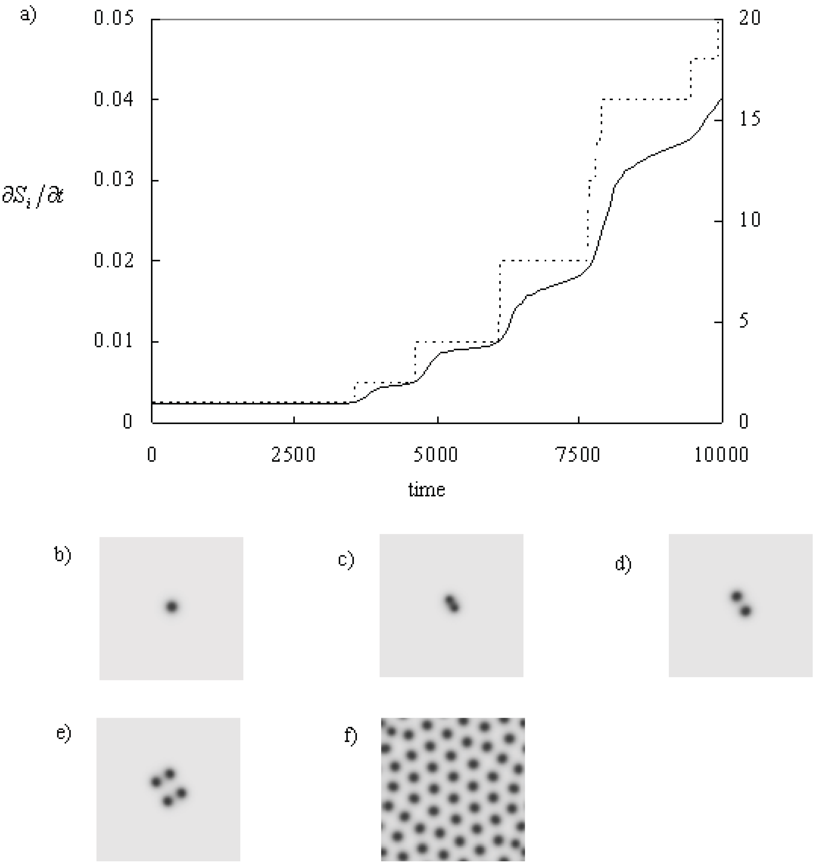
In this section, the relations between the pattern formation and the entropy production are described. These relations are discussed in the cases of self-replicating spots and line pattern formation. Figure 2 shows the self-replicating process of a spot. A circular spot becomes unstable to become a peanut shape [15]. Then, the spot is divided into two. The number of spots doubles: 1,2,4, and so on. Finally, spots fill the whole space, and the system becomes static. At the beginning, the entropy production increases rapidly during the self-replicating process. On the other hand, this quantity increases slowly when the spots looks static. It means that the entropy production increases almost proportional to the number of the spots. Finally, it becomes stable when the system shows static pattern [30].

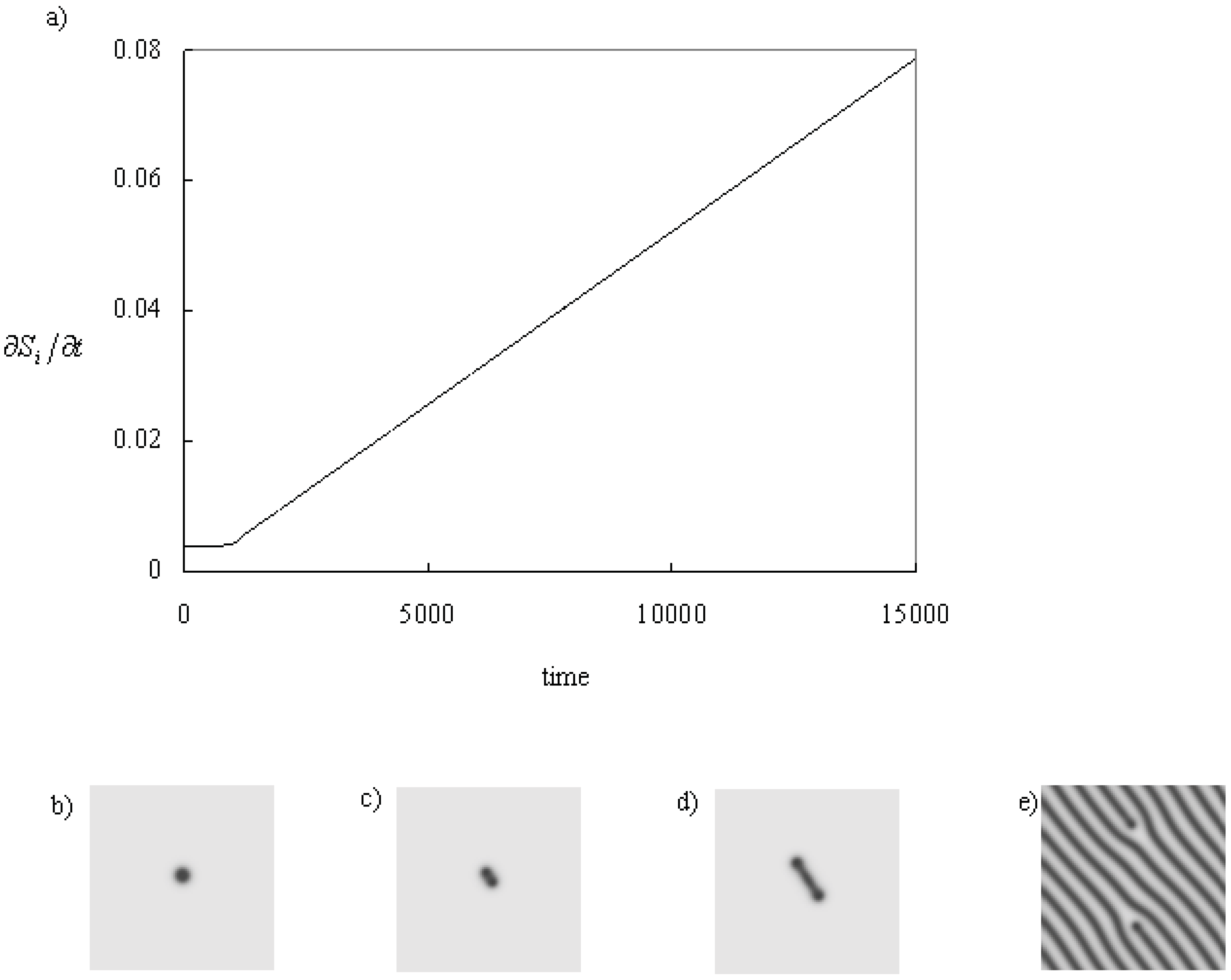
Figure 3 shows the process in which a line develops from a spot. As same in the previous example, a spot becomes unstable to be a peanut shape; however, it does not self-replicate. The heads of the peanut move apart from the each other and a line remains between them. The stretching speed of the line is constant, and the entropy production increases constant velocity while there is no obstacles (the boundary and other patterns). Finally, the line fills the system, and the system becomes static, and the entropy production becomes constant.

Figure 2. Time series of the entropy production and pattern when the system shows self-replicating spots. The parameters: f = 0.025 k = 0.064, and k_r = 0.001. (a) Time series of the entropy production. Line: entropy production, dotted line: the number of the minima of U (~ spots). (b) Initial spot pattern at t = 0.0. (c) The spot becomes a peanut shape which has two minima (t = 3,700.0). (d) The peanut shape becomes two spots, t = 4,000.0. (e) The two spots becomes four spots, t = 5000.0. (f) The spots fill the system (the final state, t = 20,000.0). Time and space resolutions are dt = 0.25 and dx,dy = 0.005, respectively. The system size is 256 x 256 grids and the periodic boundary conditions are applied.

Figure 2. Time series of the entropy production and pattern when the system shows self-replicating spots. The parameters: f = 0.025 k = 0.064, and k_r = 0.001. (a) Time series of the entropy production. Line: entropy production, dotted line: the number of the minima of U (~ spots). (b) Initial spot pattern at t = 0.0. (c) The spot becomes a peanut shape which has two minima (t = 3,700.0). (d) The peanut shape becomes two spots, t = 4,000.0. (e) The two spots becomes four spots, t = 5000.0. (f) The spots fill the system (the final state, t = 20,000.0). Time and space resolutions are dt = 0.25 and dx,dy = 0.005, respectively. The system size is 256 x 256 grids and the periodic boundary conditions are applied.

From the above results, we conclude that the value of the entropy production is proportional to the pattern density, and the entropy production can be an index of pattern formation. Because of this feature, the entropy production is a smooth function of the parameters in the parameter region where pattern morphology is preserved. On the other hand, the entropy production changes in a discontinuous manner when the pattern morphology changes drastically, e.g., the spot pattern changes to the line pattern. Therefore, we can show the parameter regions of the patterns by using the entropy production. Here, we show these parameter regions with this quantity when the system has bistability. 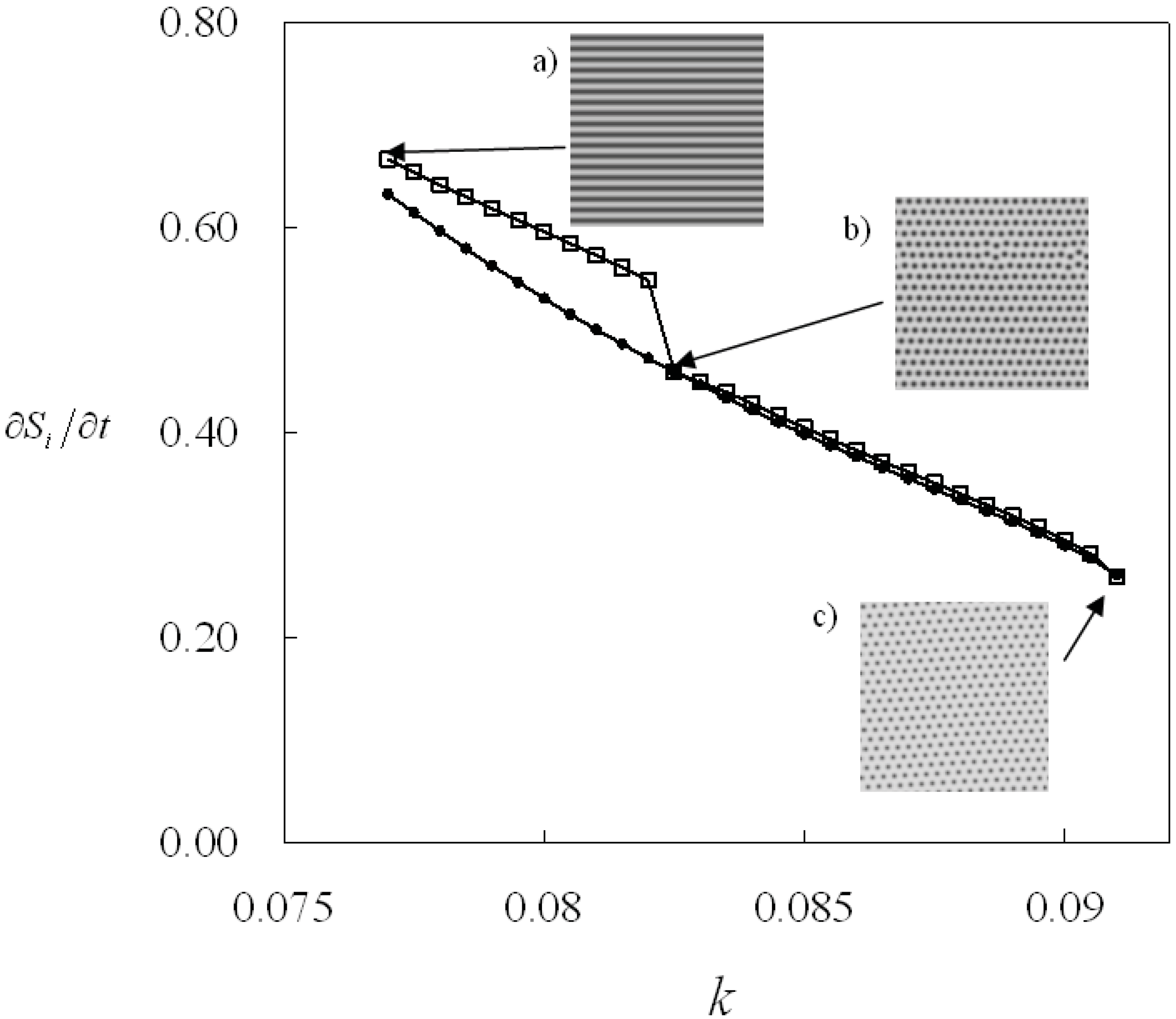Figure 4 shows the change of the entropy production as the parameter k is incremented and decremented. The system shows the spot pattern in the parameter region 0.077 ≤ k ≤ 0.082 and the line pattern in the parameter region 0.0825 ≤ k ≤ 0.091 as k is incremented. In this case, the entropy production changes discontinuously at the parameter k = 0.0825. On the other hand, the system shows only the spot pattern in the region 0.077 ≤ k ≤ 0.091 as k decreases. Then the entropy production increases smoothly in this case. As a result, the entropy production shows two values in the parameter region 0.077 ≤ k ≤ 0.082 where the system shows bistability. Therefore, the entropy production can be an indicator to distinguish the parameter regions of the patterns [31].

These results suggest that the minimum value of entropy production does not necessarily mean the implementation of the most stable state. The r-GS model shows bistability of patterns, so the entropy production shows different values even under the same parameter conditions. Thus the entropy production is not an index of pattern selection and does not play the role of a global thermodynamic potential, i.e., a Lyapunov function. It is probably because the entropy production is the time derivative of the entropy that is produced inside the system only, and the interaction between the system and its environment is not taken into account.

Figure 3. Time series of the entropy production and pattern when a line is stretching. The parameters: f = 0.048 k = 0.066 k_r = 0.001. (a) Time series of the entropy production. (b) A spot at the initial state, t = 0.0. (c) The spot becomes a peanut shape, t = 1,100.0. (d) The heads of the peanut move apart from each other and the line is stretching, t = 2,000.0. (e) The final state where the line fills the system, t = 200,000.0. The calculation conditions are the same in Figure 2.

Figure 3. Time series of the entropy production and pattern when a line is stretching. The parameters: f = 0.048 k = 0.066 k_r = 0.001. (a) Time series of the entropy production. (b) A spot at the initial state, t = 0.0. (c) The spot becomes a peanut shape, t = 1,100.0. (d) The heads of the peanut move apart from each other and the line is stretching, t = 2,000.0. (e) The final state where the line fills the system, t = 200,000.0. The calculation conditions are the same in Figure 2.

Figure 4. Entropy production is shown as a function of the parameter: k at f = 0.04 and k_r = 0.01. The bistability region of the lines and the spots pattern. Open square: The parameter k is incremented from k = 0.077. The initial stripe pattern is inserted as (a), at k = 0.077. The pattern changes into spots pattern (b) at k= 0.0825. Dot: The parameter k is decreased from k = 0.091. The initial pattern is inserted as (c). The pattern morphology does not change in this case.

Figure 4. Entropy production is shown as a function of the parameter: k at f = 0.04 and k_r = 0.01. The bistability region of the lines and the spots pattern. Open square: The parameter k is incremented from k = 0.077. The initial stripe pattern is inserted as (a), at k = 0.077. The pattern changes into spots pattern (b) at k= 0.0825. Dot: The parameter k is decreased from k = 0.091. The initial pattern is inserted as (c). The pattern morphology does not change in this case.

5. Calculation of Entropy Balance Equation

5.1. Definition of the Entropy Flow

For calculation of the entropy balance equation, the divergence of the entropy flow should be calculated. This term can be written as an integral over the system surface Ω with the divergence theorem:

$$\frac{\partial S_e}{\partial t}={\displaystyle {\int }_V(-\mathrm{div}\mathbf{\text{J}})dV}={\displaystyle {\int }_{\Omega }{\displaystyle \sum _j\frac{{\mu }_j}{T}{j}_j\cdot nd}\Omega }$$

(6)

where n is the unit vector normal on the system surface. μ_j and j_j are the chemical potential and the flux vector of the jth chemical species, respectively. The chemical potential of the jth chemical species is defined as:

$${\mu }_j={\mu }_j^{*}+k_{B}T\ln c_j,$$

(7)

where μ_j^* is the standard chemical potential and c_j is the concentration of the jth chemical species [1,2]. The standard chemical potential has a constant value characteristic for each chemical species.

5.2. Description of the Flux Vector and the Chemical Potential

For the calculation of the entropy flow, the flow vector j and the chemical potential μ in Equation 6 should be described concretely. Here, descriptions of these quantities in the present model will be given.

The mass flow vectors are derived from the system configurations. Here, we consider a one-dimensional reaction-diffusion system for simplicity [31]. Spatial imhomogeneity in concentrations appears along one direction x only (In Figure 5, the system lines along the vertical direction). From the equations of the system, the flow vector j is described; Inward flows of chemical species are given as:

$$j_U=-f{\mathbf{e}}_z,j_W=0,j_P=0,$$

(8)

and the outbound flows are given as:

$$j_U=fU{\mathbf{e}}_z,j_W=fW{\mathbf{e}}_z,j_P=fP{\mathbf{e}}_z,$$

(9)

where e_z is the unit vector directed parallel to the surface normal vector. Here, the direction of this vector is perpendicular to the direction x. The flow terms are set to zero at the Neumann boundary conditions [31].

The chemical potential is described with the concentrations of the chemical species and its standard chemical potential. However, we face a problem that the values of the standard chemical potentials are unknown in our model. This fact means that it is impossible to calculate the entropy flow from Equations 6 and 7. To avoid this inconvenience, we introduce an alternative chemical potential, μ_r, which is called the relative chemical potential [31].

The relative chemical potential is defined as:

$${\mu }_{r,j}={\mu }_j^{*}+k_{B}T\ln c_j-{\mu }_j^{*}-k_{B}T\ln c_{e,j}=k_{B}T\ln \frac{c_j}{c_{e,j}},$$

(10)

where c_e,j is the concentration of the jth chemical species at the equilibrium state. This potential means that the base of the potential is moved from the constant value (the standard chemical potential which is defined by Gibbs) to the equilibrium state of the system. This equilibrium state is defined as the steady state to which the non-equilibrium system should reach if the system is suddenly isolated from its environment.

For the calculation of the relative chemical potentials in the present system, the equilibrium state c_e,j (=c_e,j(t)) is calculated from the following three equations. These equations are obtained by assuming that the system is isolated, i.e., f = 0.0:

$${\displaystyle \int \left(U+W+P\right)dV=\left(U_e+W_e+P_e\right)V},$$

(11)

$$U_e{W}_e^2=k_r{W}_e^3,$$

(12)

$$k{W}_e=k_r{P}_e,$$

(13)

where V is the volume of the system; U_e, W_e and P_e are the equilibrium concentrations of chemical species U, W and P, respectively. The first equation means that the total number of molecules is preserved in the r-GS model.

5.3. Results

In order to discuss the relation between the entropy balance and pattern, the thermodynamic quantities are calculated for a propagating and reflecting pulse wave in the one-dimensional system.

Figure 5. Time series of the pattern and the thermodynamic quantities: the entropy production, the entropy flow and the entropy change. The parameters: f = 0.01 k = 0.047 k_r = 0.001. The top panel shows the propagating pulse. The horizontal and the vertical axes represent time and space, respectively. A black pulse reflects at the Neumann boundary. The second, the third and the forth panels show the entropy production, the divergence of entropy flow and the entropy change, respectively. Time and space resolutions are dt = 0.1 and dx = 0.005, and the system size is 800dx.

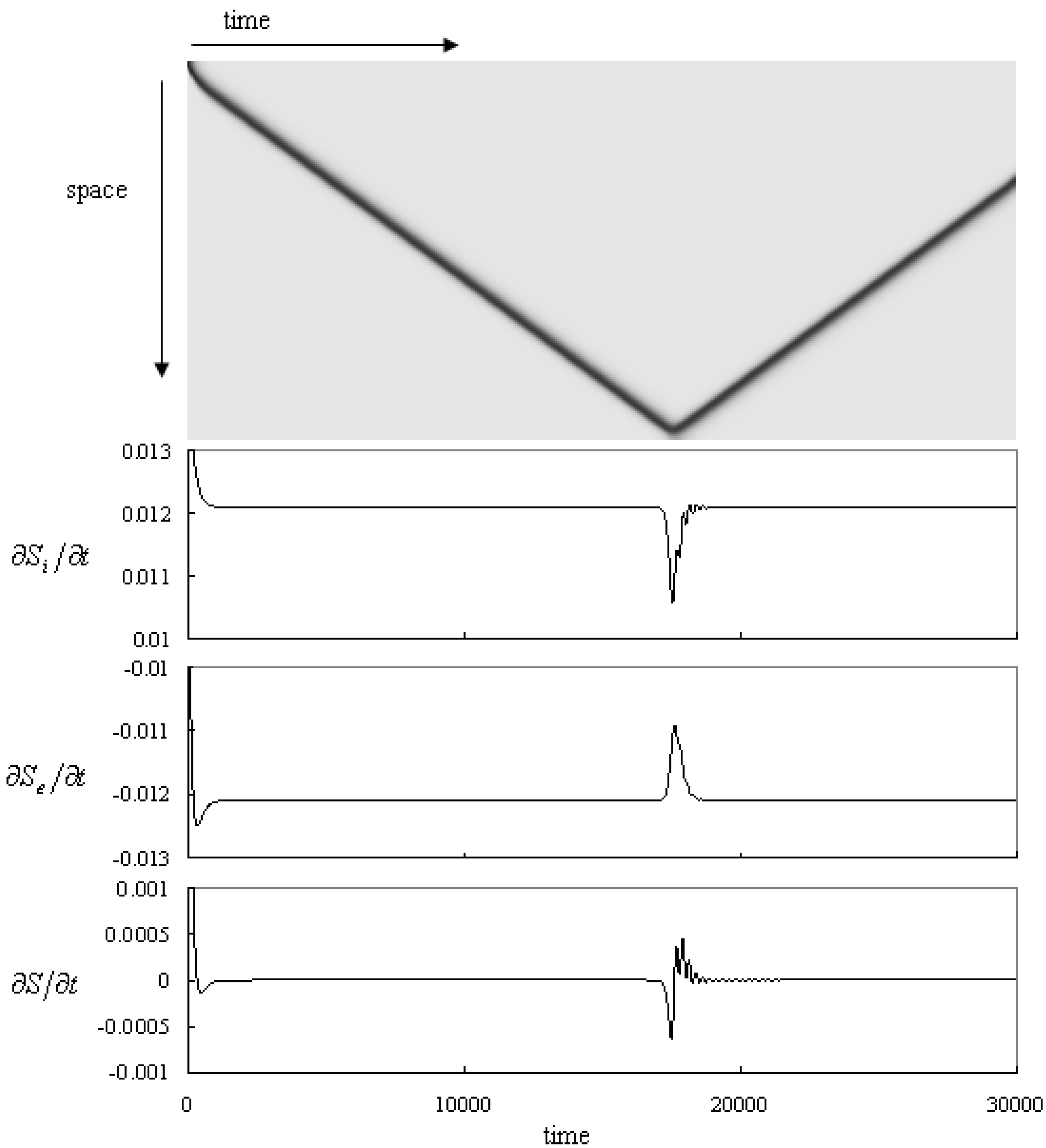
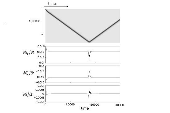
Figure 5. Time series of the pattern and the thermodynamic quantities: the entropy production, the entropy flow and the entropy change. The parameters: f = 0.01 k = 0.047 k_r = 0.001. The top panel shows the propagating pulse. The horizontal and the vertical axes represent time and space, respectively. A black pulse reflects at the Neumann boundary. The second, the third and the forth panels show the entropy production, the divergence of entropy flow and the entropy change, respectively. Time and space resolutions are dt = 0.1 and dx = 0.005, and the system size is 800dx.

The time series of the system is shown in the upper panel of Figure 5. The system is set to the fixed point (U,V, P) = (1.0, 0.0, 0.0) homogeneously, then perturbed initially to (0.5, 0.25, 0.0) at the upper side (10 calculation grids) of the system. A pulse wave propagates to the other side from the perturbed area with a constant velocity. When the pulse reaches the bottom side, the pulse reflects to propagate back to the upper side. As this pulse reflection occurs repeatedly at the Neumann boundaries, the pulse propagates back and forth between the boundaries.

The time series of the thermodynamic quantities are shown in Figure 5 (lower panel). The entropy production shows a constant value after the pulse is initiated. This value does not change until the pulse reaches the boundary. It decreases when the pulse reaches near the boundary and goes back to the constant value after the reflection. Thus, it behaves like a damping oscillation.

The absolute value of the entropy flow is the same as that of the entropy production while the pulse is propagating steadily. This quantity begins to increase when the pulse reaches near the boundary. Similar to the previous case, this quantity goes back to the constant value with a damping oscillating behavior after the reflection. After that, this value becomes the constant value, too. It looks that the absolute value of this quantity follows the value of the entropy production except that the amplitude of the dumping oscillation is smaller than that of the entropy production.

The entropy change converges to zero initially and it becomes zero while the pulse propagates constantly. This quantity decreases and becomes negative values when the pulse reaches near the boundary. The entropy change goes up to be a positive value at the moment of the reflection. After that, it reaches to the zero constant with the dumping oscillating behavior. This quantity becomes zero again and the pulse propagates with a constant velocity to the opposite side.

5.4. Discussion

The entropy production is roughly proportional to the black region in the pattern, as shown in Section 3. The entropy change shows a constant value when the pulse propagates with constant velocity and when its profile is kept constant. It means that the entropy production is constant if the shape of the pattern is independent of time, i.e., it does not depend whether the pattern is static or traveling constantly. On the other hand, the entropy production slightly changes while the pulse is reflecting. The reason for this change is that the shape of the pulse is deforming during the reflection process. Actually, the minimum value of the pulse profile slightly increases from 0.259 to 0.289 at the moment when the pulse reflects. After the reflection, the pulse shows breathing behavior with damping and then the thermodynamic quantities show some fluctuations during the reflecting process.

The negative value of the entropy flow represents that the excess amount of the entropy is thrown out to the environment through the mass flow. The absolute value of the entropy flow is almost the same as that of the entropy production. Therefore, the absolute value of the entropy change is smaller than 1/10 of these values. This means that most of the entropy produced inside the system is thrown out to the environment. Especially when the system shows a propagating pulse with a constant velocity, the entropy change is zero. This property is the same as that when the system shows a static pattern [31]. Therefore the entropy production balances with the entropy flow if the profile of the pattern is kept constant and then this property does not depend whether the pattern stays or moves constantly.

The entropy change shows non-zero values during the pattern development [22]. It shows also non-zero values while the pulse is reflecting, i.e., the shape of the pulse is deforming. It shows both negative and positive values during this process. The time integration of the entropy change over this process becomes zero. This means that the entropy shows the same values before and after the reflection of pulse. In this case, both the velocity and the shape of the pulse are preserved before and after the reflection. This calculation indicates that the entropy of the system shows the same value if the system shows the same pattern profile.

The entropy change is calculated with the relative chemical potentials. These potentials are based on the state of the system and not on the standard chemical potentials, which are unique constants for each chemical species. Despite this, the properties of the entropy change in our calculation coincide with the two properties of the entropy which are deduced from the intrinsic property of the entropy as a state function of the system. One is that the entropy change becomes zero, i.e., the entropy shows a constant value if the state (pattern shape) of the system is not time dependent. The behavior is evident by the above-mentioned calculations for of the pulse propagating with a constant velocity. The other is that the entropy is a unique function of the state of the system. This property is shown by the fact that the entropy of the system is the same before and after the pulse reflection. Therefore, we expect the thermodynamic quantity calculated with the relative chemical potential can be useful to discuss the thermodynamic behavior of the non-equilibrium system and its properties are consistent with the established properties of entropy.

6. Summary

In this review, the relations between the thermodynamic quantities and pattern formation are investigated in a reaction-diffusion system composed of the reversible Gray-Scott model. First it is shown the relation between the entropy production and the pattern formations. The results of two examples indicate that the entropy production is proportional to the area of the black region of the system. Thus, the entropy production could be used as a quantitative index of patterns. An example is give to show the existence of the parameter region where the system has a bistability by using this quantity as a measure.

The relative chemical potential is introduced in order to calculate the entropy balance in a non-equilibrium dissipative system. The entropy balance of the propagating pulse is calculated with this potential in the one-dimensional reaction-diffusion system. The thermodynamic quantities show constant values while the profile of the pulse is time independent. This thermodynamic feature is the same as in the case where the system shows a static pattern [31]. Therefore, the thermodynamic quantities should be constant if the pattern profile is independent of time, even though it moves constantly. This feature coincides with a property of entropy that it does not change while the state of the system does not change. We also calculate the time integration of the entropy change during the reflection of pulse and deduce that the entropy before and after the pulse reflection takes the same value. This fact is coincident with such an attribute of entropy that the entropy is a unique function of the state of the system. Therefore, we believe that the thermodynamic quantities can be calculated appropriately by using the relative chemical potential.