Statistical Vibroacoustics and Entropy Concept

Abstract

Statistical vibroacoustics, also called statistical energy analysis (SEA) in the field of engineering, is born from the application of statistical physics concepts to the study of random vibration in mechanical and acoustical systems. This article is a discussion on the thermodynamic foundation for that approach with particular emphasis devoted to the meaning of entropy, a concept missing in SEA. The theory focuses on vibration confined to the audio frequency range. In this frequency band, heat is defined as random vibration that is disordered vibration and temperature is the vibration energy per mode. Always in this frequency band, the concept of entropy is introduced and its meaning and role in vibroacoustics are enlightened, together with the related evolutionary equation. It is shown that statistical vibroacoustics is non-equilibrium thermodynamics applied to the audio range.

1. Motivation for Statistical Vibroacoustics

Vibracoustics is the science of structural waves, acoustical waves and their interaction. Presented in classical textbooks, vibroacoustics is usually divided into the study of propagation of waves, natural modes, radiation of sound, sound transparency and structural response. This science is at the interface of acoustics and elastodynamics that is the theories of propagation of small perturbations in fluids and solids. As such, vibroacoustics focuses on the coupling between structural and acoustical waves. Vibroacoustics is fully operative for prediction and control of systems as well as it explains in a satisfactory way all phenomena within its range of application. This is a well-known theory daily applied in science and engineering and whose foundations are well-established. In that sense, vibroacoustics could be considered as finished from the theoretical point of view.

The investigation of the governing equations of vibrating structures and acoustics began in the eightieth century with the study of string vibration by d’Alembert and beams by Euler and Bernoulli. During the nineteenth century and the early of the twentieth century, the governing equations for almost all simple vibrating systems have been derived, plates by Germain, beams with shear effect by Timoshenko, shells by Donnell, high order plate theory by Mindlin but with many other contributors such as Helmholtz, Kirchhoff, Rayleigh, Sommerfeld, Love, Lamb and many others. The famous Rayleigh’s treatise, The Theory of Sound, published in 1894 for the second edition and always available in bookstores [1], gives a precise idea of what was the state of the art at the end of the ninetieth century.

But the solving of the governing equations more specifically with fluid-structure interaction, is relatively more recent. Indeed, some of these solutions for pure structural or acoustical problems are very old. The discovery of propagative solutions in strings and their normal modes makes strings the first example of vibrating structure entirely solved. But closed-form solutions for sound radiation or structural response have been discovered up to the seventies. In this concern, the introduction of complex analysis methods and in particular the Wiener-Hopf method led to significant advances. For instance, Crighton [2] solved the problem of an acoustical spherical wave impinging an infinite membrane and Davies [3] the problem of sound radiation of semi-infinite membranes. Many other canonical problems of vibroacoustics were solved with the wave approach and the power of complex analysis. In the case of finite structures, the modal approach has been shown to be more appropriate. The major advance was to recognize that sound radiation is mainly due to edges, corners and other singularities. Jointly with these two approaches, wave method for infinite or semi-infinite problems and modal decomposition for finite structures, almost all canonical problems of sound radiation and structural response have been solved either with exact or approximated solutions.

The eighties are the period of numerical developments. The development of finite element softwares gave a decisive advantage to the modal approach. The computation of eigenfrequencies and eigenmodes of complex structures, that is not possible by hand beyond simplest geometries, is numerically reducible to a common problem of linear algebra. Indeed, computers are the best tool to solve large linear sets of equations. This is why a race for power has been engaged for these three last decades. During the eighties, the number of degrees of freedom that was manageable on strongest computers was only about few hundreds of thousand. It was about the million during the nineties while it is now common to solve problems with one dozen of million degrees of freedom.

The duality of wave and modal approaches is somewhat general. But beyond the case of infinite or semi-infinite geometries where the wave approach is the only one applicable giving analytical solutions, the systematic use of computers has given credence to the idea that the modal approach is the only one efficient in practice. Most of problems can be solved by the modal approach (we do not discuss the mathematical conditions for the existence of a modal basis, but say that structures and acoustical cavities are finite). From the knowledge of eigenmodes, it is possible to compute the response of system to any excitation, in both time and frequency domain. We could say roughly that the behaviour of vibroacoustical systems is reducible to the knowledge of their modal basis. Therefore, in practice, the only difficulty is to compute the modal basis that is well-done by computers.

But this approach by the ’brute force’ has three limitations.

First of all, the mathematical condition for convergence of finite element method imposes a fixed number of degrees of freedom per wavelength (in practice seven is considered satisfactory). But, when the frequency of analysis increases, the wavelength decreases therefore the total number of degrees of freedom increases drastically. Since computers have a limited capacity, no computation is possible beyond a certain limit frequency. Nowadays, this limit is not so high (Table 1) in regards to the audio frequency range 20 Hz–20 kHz.

Table 1. Typical values of maximum frequency for a finite element model of order of several millions degrees of freedom.

automotive	500 Hz
aircraft	50 Hz
large ship	10 Hz
launcher	1 Hz

Table 1. Typical values of maximum frequency for a finite element model of order of several millions degrees of freedom.

automotive	500 Hz
aircraft	50 Hz
large ship	10 Hz
launcher	1 Hz

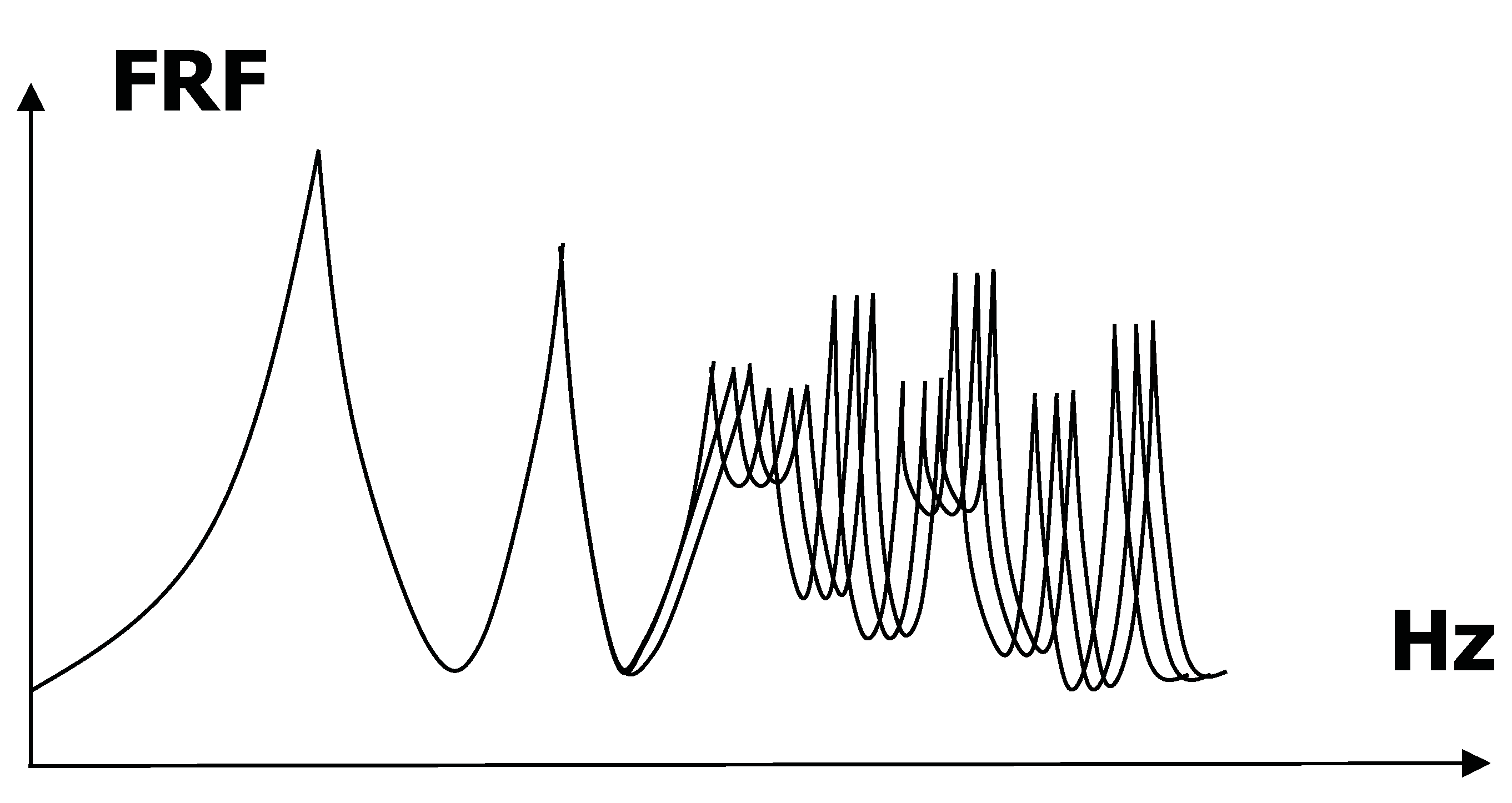
The second limitation is concerned with modal overlap. Modal overlap is a measure of the overlapping of successive modes. If the resonance peaks of two successive modes in the frequency response function are clearly separated, the modal overlap is low. But if the peaks are closed meaning that the valley between them is not deep, the modal overlap is high (Figure 1). In the extreme case of a very large modal overlap, peaks can totally vanish and the frequency response function is smooth. Modes exist but are not visible. They cannot be distinguished by a modal analysis and their utility is therefore questionable. Why to spend so much effort in calculating the modes which individually do not influence the response of system?

The third limitation is about the amount of available information. When the number of modes is large, the results provided by finite element softwares i.e., values of natural frequencies, mode shapes and the repartition of vibration among them, become sensitive to small modifications of the model (Figure 2). And indeed, nothing can be known exactly. This sensibility to details has also been observed on actual population of similar systems [4]. In this case, probability or alternative theories such as info-gap approach are unavoidable [5]. The raised question is the following one. Even if we wait for the venue of super large computer (Moore’s law which is valid for several decades now, tells us that the capacity of computers is just a question of time), what to do with a so large amount of information? Is-it realistic to consider that the knowledge of natural frequencies is relevant to predict the behaviour of vibroacoustical systems?

For these three reasons, the modal approach fails when the frequency of analysis is too high. This is why an alternative statistical approach called statistical energy analysis, has been developed in vibroacoustics.

Figure 1. Modal density n-modal overlap M. Typical shapes of frequency response function for large modal density n >> 1 and large modal overlap M >> 1.

Figure 1. Modal density n-modal overlap M. Typical shapes of frequency response function for large modal density n >> 1 and large modal overlap M >> 1.

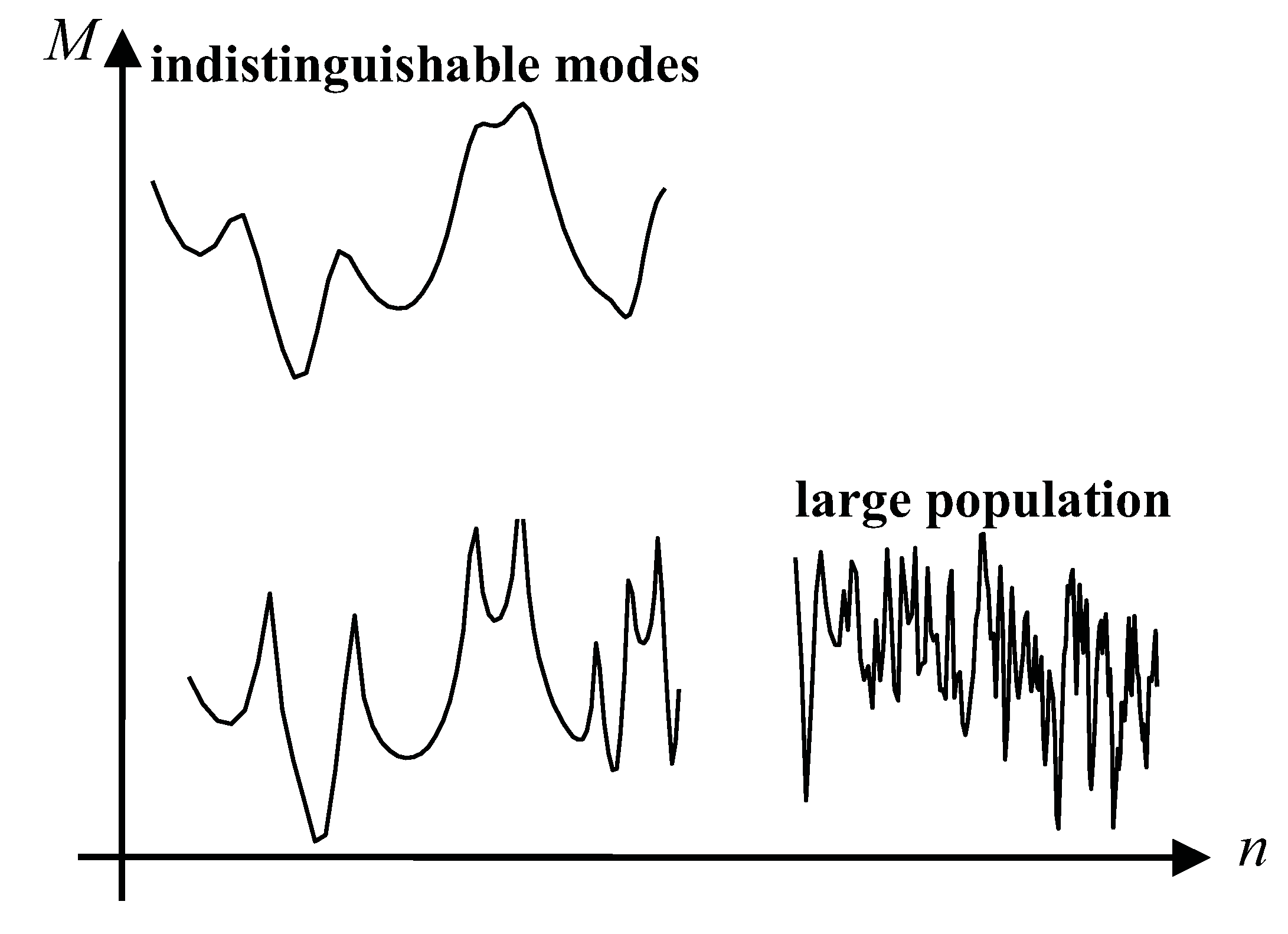
Figure 2. Sensitivity of frequency response function to details of model. Numerical models are reliable at low frequency but become sensitive to small fluctuations at high frequency.

Figure 2. Sensitivity of frequency response function to details of model. Numerical models are reliable at low frequency but become sensitive to small fluctuations at high frequency.

2. Statistical Energy Analysis

Statistical energy analysis (SEA) is born from the application of statistical physics concepts to vibroacoustics [6]. Elaborated during the sixties, this theory lies on a simple idea: When the number of modes in vibroacoustical systems is so large that the solving of governing equations becomes unrealistic, it is preferable to give up a deterministic description of the system and to adopt a statistical point of view.

However, the application of statistical method to a particular field of physics is usually not sufficient to automatically obtain an effective theory. The use of statistics must be justified by the existence of a collective behaviour of the physical system, something like an empirical law observable at macroscopic scale. This law usually stems from the complexity of the behaviour of large populations. And in the same time, this law must not hold for single individual otherwise the statistical assumption would not add anything else that we ever know. The general problem is to introduce one or several macroscopic variables whose behaviour is statistically simple. For instance, in the kinetic theory of gases, temperature and pressure play the role of these macroscopic variables and the law of perfect gases expresses a simple collective behaviour.

In the special case of vibroacoustics, the key result was to recognize that the energy transfer between mechanical oscillators is considerably simplified when excitation forces are random processes. The canonical problem is the following one: Two mechanical oscillators with stiffness k_i, mass m_i and viscous damping c_i where i = 1, 2 are excited by external random forces f_i(t). They dissipate energy in dashpots but they also exchange mechanical power through a coupling spring K as shown in Figure 3. It has been demonstrated [7,8,9,10] that in such a situation the power being exchanged between two oscillators is proportional to the difference of vibrational energies. That is,

$$P_{12}=g\left(E_1-E_2\right),$$

(1)

where g is a function of mechanical parameters k_i, m_i, c_i and K. Indeed this result is not true in its strict sense but only in a statistical sense. External forces f_i(t) must be stationary random processes with zero means, white noise (constant power spectral density) and mutually uncorrelated (zero cross-correlation function). The coupling must be light K << k_i [11] and conservative [12]. Under these assumptions, Equation (1) is valid provided that E_i and P_ij are respectively the statistical average of vibrational energies and transmitted power.

Figure 3. Energy exchange between two mechanical oscillators. For random, stationary, uncorrelated and white noise forces and for light and conservative coupling, the exchanged power is proportional to the difference of vibrational energies.

Figure 3. Energy exchange between two mechanical oscillators. For random, stationary, uncorrelated and white noise forces and for light and conservative coupling, the exchanged power is proportional to the difference of vibrational energies.

The second ingredient in the development of statistical vibroacoustics was that this simple proportionality also holds for multi-modal systems provided that the vibrational energies are substituted with the modal energies i.e., the vibrational energy E_i divided by the number of modes N_i [13].

$$P_{12}=g^{\prime }\left(\frac{E_1}{N_1}-\frac{E_2}{N_2}\right),$$

(2)

where N_i is the number of modes within sub-system i. The coefficient g′ is a function of all mechanical parameters and is conventionally written as,

$$g^{\prime }=\omega N_1{\eta }_{12}=\omega N_2{\eta }_{21}$$

(3)

where ω is the average frequency of modes and η_ij is the so-called coupling loss factor. The generalization of the single degree of freedom Equation (1) to the multiple degrees of freedom Equation (2) is a direct consequence of equipartition of vibrational energy within sub-systems (Figure 4). This the key point of the proof. Equipartition of vibrational energy among modes of same sub-systems naturally appears under certain conditions [14,15,16] and is therefore not an additional assumption. The thermal equilibrium is reached in each sub-system. But Equation (2) tells us more. Vibrational power flows through the light coupling proportionally to the difference of modal energies. So, by analogy with thermics, if the modal energy is called ‘vibrational temperature’, Equation (2) is a linear relationship on power flow and temperatures for adjacent sub-systems which have not the same temperature i.e., which are not in mutual equilibrium. This is therefore an analogy with linear non-equilibrium thermodynamics.

Figure 4. Energy exchange between two groups of degrees of freedom. All modes of first sub-system exchange energy with all modes of second sub-system. When equipartition of energy is fulfilled, the net power exchanged between sub-systems is proportional to the difference of modal vibrational energy.

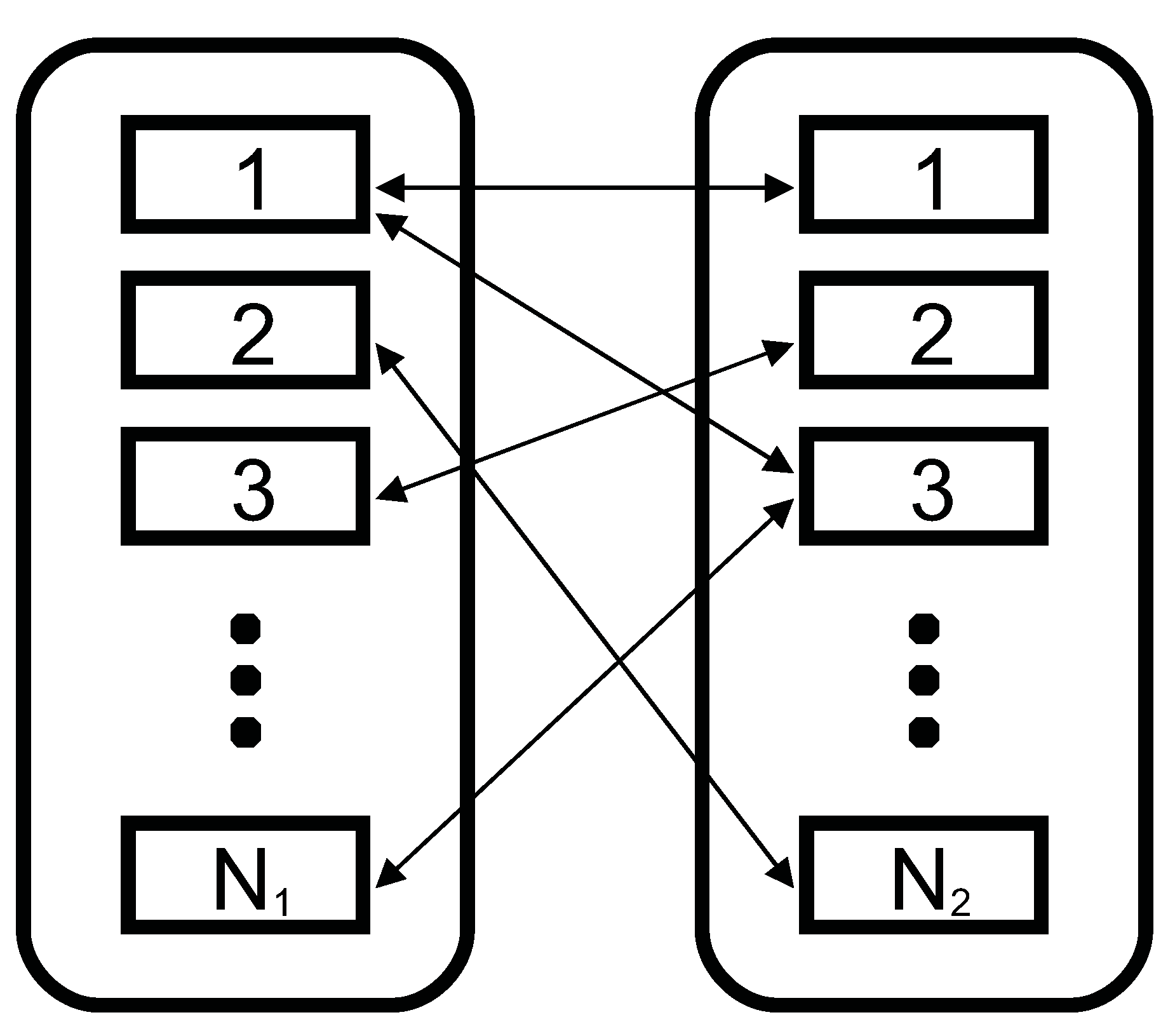
Figure 4. Energy exchange between two groups of degrees of freedom. All modes of first sub-system exchange energy with all modes of second sub-system. When equipartition of energy is fulfilled, the net power exchanged between sub-systems is proportional to the difference of modal vibrational energy.

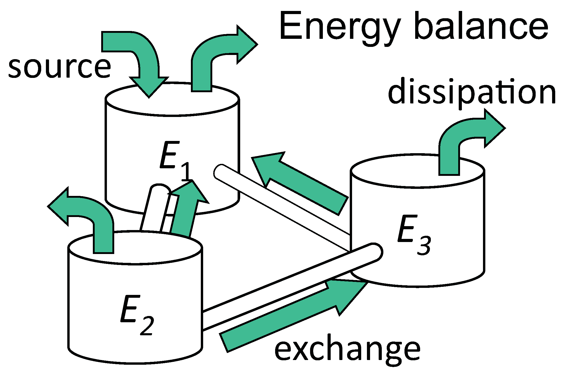
The most important consequence of the statistical law Equation (2) is that it allows a description of vibroacoustical systems entirely in terms of energy. In steady-state condition, the energy balance of sub-system i is,

$$P_i=\omega {\eta }_i{E}_i+\sum _{j\ne i}\left(\omega {\eta }_{ij}{E}_i-\omega {\eta }_{ji}{E}_j\right)$$

(4)

where P_i is the vibrational power being injected in sub-system i by external sources, ωη_iE_i the power being dissipated by internal losses with various physical origins summarized in the damping loss factor η_i and ωη_ijE_i − ωη_jiE_j is the net power being exchanged with other sub-systems. The energy balance Equation (4) is nothing else than the first principle of thermodynamics applied to vibration confined in the audio frequency range. The principle of statistical energy analysis is summarized in Figure 5. The complex structure is split in sub-systems constituted of mode group equitably sharing vibrational energy and lightly coupled with each others.

Figure 5. Principle of statistical energy analysis. The complex structure is subdivided in sub-systems containing vibrational energy. Sub-systems can receive power from external sources, dissipate energy by internal losses and exchange energy with neighbour sub-systems proportionally with the difference of modal energies.

Figure 5. Principle of statistical energy analysis. The complex structure is subdivided in sub-systems containing vibrational energy. Sub-systems can receive power from external sources, dissipate energy by internal losses and exchange energy with neighbour sub-systems proportionally with the difference of modal energies.

Equation (4) is of a great practical interest. It allows the prediction of mean vibrational energy of sub-systems E_i provided that injected powers P_i are known, without solving the governing equations of the entire system. The gain is huge. Instead of dealing with N modes where N can be of order of several millions [17], we deal with n sub-systems where n is considerably lower than N, usually only a couple of dozens. The solving of the set of linear equations resulting from the finite element model of order ∼7N is substituted by the solving the set of n linear equations of Equation (4). In practice, sub-systems are structural components of the system such as beams, plates, shells, acoustical cavities and so on. During the last decades, the method has been applied in almost all fields of engineering: automotive industry, shipbuilding [18], civil engineering [19], acoustical isolation [20] and so on. Indeed, the main difficulty is to choose the sub-systems and in particular to do it in such a way that the light coupling assumption is not violated and that the equipartition of energy is verified in all sub-systems. The second difficulty is to obtain efficient relationships of coupling loss factors η_ij [21,22]. There is an extensive literature on the subject of coupling loss factors in various situations, plate-plate coupling, room-plate, beam-plate and much more. The method also allows an easy determination of energy flow paths [23] and it exists is a closed connection with ray-tracing [24]. But, instead of discussing the practical interest and difficulties of statistical energy analysis [25], the rest of the paper focused on a discussion on the meaning of such an approach and in particular to clarify the analogy with non-equilibrium thermodynamics.

3. Entropy in Statistical Vibroacoustics

The theoretical presentation of statistical vibroacoustics of previous section could be considered as sufficient from the practical point of view. The statistical law Equation (2) can be derived directly from the equations of mechanical oscillators and some suitable approximations. The obtained energy balance Equation (4) is closed so that any further equation is required. The system is entirely described in terms of vibrational energies and exchanged powers. In that sense, Equation (4) and therefore statistical energy analysis constitutes a self-sufficient theory of randomly excited mechanical oscillators. Equation (4) provides an efficient tool to predict the behaviour of systems and even to control them. From the point of view of engineering, all the required material is available. Apart from the problem of the effective determination of the coupling loss factors η_ij and their applicability for actual structures, the theoretical development of statistical vibroacoustics could be stopped here.

But this point of view is limited to the practical interest and does not raise the question of the meaning of such an approach. In this concern, the presentation of statistical energy analysis would not be complete without introducing the appropriate entropy concept and the second principle of thermodynamics. The occurrence of entropy in statistical energy analysis is not only a logical requirement for a complete and coherent derivation of statistical vibroacoustics, but it is also necessary to understand the exact link between statistical energy analysis and non-equilibrium thermodynamics beyond their apparent analogy [26,27].

To introduce entropy in statistical vibroacoustics, we must first specify the dynamical system. A sub-system is a packet of N modes with increasing natural frequencies ω_i i = 1 ⋯ N. The Hamiltonian of such a dynamical system is,

$$H(q_1,\cdots ,q_N,p_1,\cdots ,p_N)=\sum _{i=1}^N\frac{m_i{\omega }_i^2}{2}{q}_i^2+\frac{1}{2m_i}{p}_i^2$$

(5)

where q_i is the modal deflection and p_i the impulsion. In phase space, the trajectory is determined by the functions q_i(t), p_i(t), i = 1 ⋯ N, solutions of the equations of motion. A microstate at time t is therefore given by the values q_i, p_i, i = 1 ⋯ N. This is what is provided by any deterministic method such as finite element method. But in statistical vibroacoustics, forces are random and it is impossible to predict the microstate. The position q₁, ⋯, q_N, p₁, ⋯, p_N becomes a random vector in phase space and we must abandon the idea of determining it exactly. The exact repartition of vibrational energy over modes is therefore not known. What is claimed in statistical energy analysis is that we are not interested in the exact repartition of vibrational energy over modes but only in the knowledge of the number of modes N and the total vibrational energy E of sub-system as shown in Figure 6. A macrostate is therefore given by the values of the total vibrational energy E and the number of modes N.

Figure 6. Sub-systems in statistical energy analysis. A microstate is determined by the repartition of vibrational energy e_i among modes i while a macrostate is the total vibrational energy E and the number of modes N.

Figure 6. Sub-systems in statistical energy analysis. A microstate is determined by the repartition of vibrational energy e_i among modes i while a macrostate is the total vibrational energy E and the number of modes N.

Another consequence of the random nature of excitations is that the energy level of individual modes is not constant. Energy is shared between modes in a random manner. And, if at a given time, a particular mode can receive much energy to the detriment of others, at the next time, it will probably receive less energy. This perpetual modification of the repartition of vibrational energy is not due to a direct exchange of energy between modes as it is the case in the kinetic theory of gases where collisions of molecules are responsible of the energy redistribution among molecules. But the important fact is that the trajectory of sub-system in phase space explores the entire surface of constant energy H(q₁, ⋯, q_N, p₁, ⋯, p_N) = E and its neighbourhood.

Thus, the situation described above comes down to a somewhat classical problem in statistical mechanics. The state of a system is only known by its probability density of presence ρ in phase space. This distribution ρ must indeed verify the normalization condition,

$$\int \rho d\Gamma =1,$$

(6)

where dΓ = dq₁ ⋯ dq_Ndp₁ ⋯ dp_N is the infinitesimal volume in phase-space. The mean vibrational energy E is,

$$\int \rho Hd\Gamma =E.$$

(7)

The entropy attached to a distribution ρ is defined by,

$$S=-k\int \rho log\left(\rho h^N\right)d\Gamma$$

(8)

The presence of Planck’s constant is necessary for dimension reason in the argument of the log function. The usual way to link this continuous definition of entropy with the discrete one, is to divide the phase space into cells of equal size h^N. The probability p_i to be in cell i is then p_i = ρh^N. For small cells, Equation (8) is then equivalent to the discrete definition of entropy S = −k∑_i p_i logp_i.

The determination of the distribution ρ stems from the application the maximum entropy principle [28], a modern version of Laplace’s principle of insufficient reason. This method to derive the canonical distribution is sometimes controversial and the debate on this question has been extensively discussed in Reference [29]. But this is not the only way to get the result and since the rest of paper focuses on the consequences of the obtained expression of entropy, we shall not discuss the philosophical justification of the maximum entropy principle. The problem is to maximize S of Equation (8) under the constraints Equations (6) and (7). It leads to the canonical distribution,

$$\rho (q_1,\cdots ,q_N,p_1,\cdots ,p_N)=\frac{exp(-\beta H)}{Z}.$$

(9)

The factors Z and β are two Lagrangian multipliers. They are respectively associated to the constraints Equations (6) and (7). The partition function Z(β) can be calculated exactly from Equations (5), (6) and (9). An approximation is,

$$Z\left(\beta \right)={\left(\frac{2\pi }{\omega \beta }\right)}^N,$$

(10)

where ω is the mean value of ω_i i = 1, ⋯ N. Introducing Equation (9) into Equation (7) yields,

$$E=-\frac{\partial }{\partial \beta }logZ\left(\beta \right),$$

(11)

The temperature T, defined from β by T = 1/kβ where k is Boltzmann’s constant, is finally calculated from Equations (10) and (11),

$$T=\frac{E}{kN},$$

(12)

which is the expected result, that is the vibrational temperature is the modal energy divided by Boltzmann’s constant k.

Let us discuss the meaning of this result. The proportionality of temperature with modal energy comes from the assumption that the canonical distribution (9) is a continuous function of phase space. This assumption is natural in the context of classical mechanics. Oscillators described by Equation (5) can take any arbitrary position in phase space. But in the context of quantum mechanics, this result would be very different. For quantum oscillators such as introduced by Planck to solve the famous black-body radiation problem, the vibrational energy can only take discrete values proportional to ℏω. Canonical distribution (9) is still valid for the allowed values of the Hamiltonian but Z(β) is now given by a discrete summation instead of an integral. The final result found by Planck is,

$$\frac{E}{N}=\frac{\hslash \omega }{exp\left(\frac{\hslash \omega }{kT}\right)-1}.$$

(13)

This law well agrees with Equation (12) for high temperature ℏω << kT as it can be seen from a first order development. But for low temperature or very high frequency, the modal energy is ℏω exp(−ℏω/kT) and the temperature is now given by a log of modal energy. In the context of vibroacoustics, typical values of vibrational energy are E ∼ 1 mJ and if we consider structure with a million of degrees of freedom N ∼ 10⁶, we get a modal energy about 10⁻⁹ J which is much larger than ℏω ∼ 10⁻³⁰ J as for a typical vibration in the audio frequency range (1 kHz). No quantum effect can be expected.

The canonical entropy is then obtained by introducing the canonical distribution Equation (9) in Equation (8) and by using the conditions Equations (6) and (7),

$$S=k\left[\beta E+log\left(\frac{Z\left(\beta \right)}{h^N}\right)\right].$$

(14)

Now, by substituting the expressions of Z and β, it yields,

$$S(E,N)=kN\left[1+log\left(\frac{2\pi E}{h\omega N}\right)\right]$$

(15)

This is the expression of the vibrational entropy of sub-system with vibrational energy E shared between N modes. E and N are two extensive quantities. A priori, both of them can vary. But if a vibrating system with a time-varying energy E(t) is meaningful, a vibrating system with a time-varying number of modes N(t) is somewhat unrealistic. It is therefore reasonable to limit the differential form dS to an energy variation dE,

$$dS=kN\frac{dE}{E}=\frac{dE}{T},$$

(16)

valid for dN = 0. This is the variation of vibrational entropy dS when vibrational energy dE is supplied to the system. This last expression well matches with Clausius’ definition of entropy if the variation of internal energy dE is interpreted as a supply of heat δQ by a reversible process.

The meaning of the key result of statistical energy analysis Equation (2) is now more apparent. The vibrational power exchanged between two adjacent sub-system is proportional to the difference of vibrational temperatures,

$$P_{ij}\propto \left(T_i-T_j\right).$$

(17)

This is a linear relationship between thermodynamic flux P_ij and the thermodynamic force T_i − T_j. The existence of such an equation from the H-theorem is discussed in next section.

4. The Role of the H-theorem in Statistical Vibroacoustics

The focus of this section is to show that vibrational entropy, through H-theorem, can provide an alternative way to approach energy method in vibroacoustics.

The starting point is the well known entropy evolution equation:

$$\frac{dS}{dt}>0.$$

(18)

that is one of the most important results both of phenomenological (Clausius) and statistical (Boltzmann) thermodynamics. Equation (18) can be conceived indeed as a phenomenological nature principle, postulated as for energy conservation. However, for it, a demonstration was originally provided by Boltzmann in his famous but also controversial so called H-theorem. Without entering the debate about controversies, here we adopt this last point of view. In fact, the H-theorem and the evolutionary property of entropy can be derived in this case in the context of Hamiltonian systems, something that allows Equation (18) to be directly transposed to vibroacoustics. Examples of entropy evolutions for some vibroacoustic systems are given in References [26,30] where it is shown Equation (18) can be applied with some care, essentially related to the hypotheses of H-theorem, if the number of degrees of freedom is large enough and/or if ensemble averages are considered.

One of the key point in developing statistical energy analysis is the use of Equation (2). However, as also mentioned in the conclusions of this paper, this is a weak point of the theory. Demonstration of Equation (2) needs some assumptions that are questionable in vibroacoustics problems. The most important is related to energy equipartitioning among the modes of the systems. The analysis of several structural and acoustic systems, shows that many different requirements must be satisfied to match equipartitioning. Among the others, the following characteristics play a role in departing or matching this ideal situation [30]: structural non-homogeneity, presence of nonlinearity, weak coupling between subsystems. This would suggest an alternative approach, that does not make direct use of Equation (2), the energy constitutive relationship, but starts indeed with Equation (18), based directly on entropy arguments.

Consider two subsystems, whose energy and entropy are E₁, S₁ and E₂, S₂, respectively. The systems are weakly coupled, such that additive properties hold for energy and entropy: total energy is just sum of the subsystems energies, because the energy stored in the coupling is negligible because of the weakness of the coupling, as well as total entropy of the system is sum of those of subcomponents. To obtain a constitutive relationship, relating energies to energy flow, as in Equation (2), the analysis of free vibrations is considered, assuming the constitutive equation is independent of the external forces. On these bases, the following relationships can be used:

• H-theorem: dS/dt > 0
• energy conservation: dE/dt = 0
• additive properties: E = E₁ + E₂, S = S₁ + S₂
• exchanged power: P₁₂ = dE₁/dt = −dE₂/dt

Simple combination of the previous equations, yields:

$$\left(\frac{d{S}_1}{d{E}_1}-\frac{d{S}_2}{d{E}_2}\right)P_{12}\ge 0$$

(19)

This result states that the power flow direction, i.e., the sign of P₁₂, depends on the sign of the difference in bracket, where each term is the gradient of entropy with respect to energy. Equation (19) shows dS_i/dE_i control the energy flow between the sub-systems. It is natural to assume the quantity dS/dE as the measure of the energy absorption capability of a system, and its inverse dE/dS as the system capability to release energy. This last is the thermodynamic temperature T of the system. Thus:

$$\frac{1}{T}=\frac{dS}{dE}$$

(20)

With this definition of T, one can assert that energy flows from the higher to the lower temperature. Equation (19) tells P₁₂ can be expressed as a function of T₁ and T₂ namely of their difference, provided that thermodynamic temperature is always positive:

$$P_{12}=f(T_1-T_2)$$

(21)

This analysis does not provide information on the form of the function f. However, using a Taylor expansion of Equation (21), about the point (T₁ − T₂) = 0:

$$P_{12}=\sum _{i=0}^N{(T_1-T_2)}^i{\left.\frac{d^{\left(i\right)}f}{d{(T_1-T_2)}^i}\right|}_{(T_1-T_2)=0}$$

(22)

Equation (22) produces a constitutive energy relationship, of which Equation (2) is just a special case obtained keeping only the first order term of the expansion, and making nought the zero-th order term to satisfy the condition P₁₂ = 0 if (T₁ − T₂) = 0. However, in Reference [31] it is shown how, in some cases, a second order expansion is required, even with the first order term equal to zero, depending on the characteristics of the analysed systems.

Note that the value of the first derivative of f in not known from the previous approach, as for Equation (2), and its determination would come from further analysis or experimental data, exactly as it happens using statistical energy analysis. The thermodynamic temperature to be used in Equation (22) in the one determined deriving Equation (15) with respect to E that produces T ∝ E/N. Thus substituting this last proportionality in Equation (22) truncated to the first order, Equation (2) is derived.

The results in this section show that one of the questionable pillars of statistical energy analysis, namely Equation (2), can be simply derived using entropy based arguments. The merit of them is not only formal, but indeed substantial, since it is recognized in this way Equation (2) is only a particular constitutive relationship belonging to a the wider family represented in Equation (22).

5. Meaning of Entropy in Statistical Vibroacoustics

The statistical method in vibroacoustics presented in the previous three sections, is applied to the audio frequency range (macroscopic vibrations) in exactly the same way that statistical mechanics is applied to thermal vibrations at the molecular scale (microscopic vibrations). The difference between statistical vibroacoustics and thermodynamics is therefore mainly a question of scale. The situation is summarized in Figure 8. Thermodynamics can be viewed as the theory of transformation of work, that is the mechanical energy with slowing varying forces (low frequency) to heat, that is vibration energy in thermal range (high frequency) while statistical vibroacoustics focuses on the only audio frequency range.

Work is the noble form of mechanical energy. It can be used to raise or move objects, to shape, to cut, to tool material, to compress gases. This is the form of energy useful in all daily mechanical actions. Heat is the ’degraded’ form of energy. This is basically also a mechanical energy but the movement is localized at the molecular scale and disordered. Work is the mechanical energy supplied to the system at the ’human’ scale that is, metre, second and kilogram, while heat is the mechanical energy supplied at the molecular scale, angstrom, femtosecond and yoctogram. With a so large spectral distance, there is no ambiguity on what is work and what is heat. The transformation of work into heat and conversely is possible but is restricted by the second principle of thermodynamics.

The transformation of work in heat is realized for instance, by friction force. In a way, the existence of friction force and more generally dissipative forces was the main motivation for the elaboration thermodynamics as a generalization of mechanics (see Reference [32] for this interesting point of view). The work δW = Fdx > 0 performed by a friction force F during the sliding dx is converted in heat δQ = δW. This conversion is accompanied by an increase of entropy dS = δQ/T > 0 (see References [33,34,35,36,37,38,39] for a review of energetic and entropic approaches in tribology). This is a transformation of energy from low frequencies to high frequencies (friction arrow in Figure 8). Another example of such a transformation is turbulence in fluid, where the energy cascade always has the same direction from low to high frequencies.

The converse mechanism from high to low frequencies is also possible. It is realized for instance by the expansion of gas. The moving piston which movement is stationary is pushed by molecules of gas with a disordered movement. The underlying process is the selection of impacts on walls which act in only one direction, those of the moving piston. This is a transformation of high frequency energy to low frequency energy (gas expansion arrow in Figure 8). In all cases, a transformation of low frequency to high frequency energy or the converse requires a highly non-linear mechanical process, shocks or friction.

In statistical vibroacoustics, the situation is different. The random vibration in the audio frequency range is our ’degraded’ form of energy and our molecules are modes. Thus, the equivalent of heat in statistical vibroacoustics is the vibrational energy randomly supplied to the system in the audio frequency range. We shall call vibrational heat and note δQ this random vibrational energy. The scales are centimetre, millisecond and gram.

If we consider the situation where all vibrational sources are random, the vibrational heat δQ > 0 is supplied to the system in such a way that its repartition over modes is not known. The increase of vibrational entropy is therefore dS = δQ/T > 0 where T = E/kN is here the vibrational temperature. Thus, a random source provides vibrational heat (random source arrow in Figure 8), warms up the system and therefore increases the vibrational entropy. This behaviour is in good agreement with classical thermodynamics.

The status of dissipation processes of vibration in statistical vibroacoustics is more interesting (damping of vibration arrow in Figure 8). The rate of dissipation of internal energy is dE = −ωηEdt where η is the damping factor. This an extraction of vibrational heat δQ = dE < 0. Therefore, the variation of vibrational entropy dS = δQ/T < 0 where T = E/kN is always the vibrational temperature, is negative. Thus, dissipation processes of vibration by reducing the vibrational level, cool down the sub-system and therefore reduce the vibrational entropy. This is exactly the converse of what happens in classical thermodynamics where dissipation processes by transforming work into heat, are the cause of irreversibility and therefore increase the thermodynamical entropy.

The transformation of thermodynamic heat in vibrational heat is also possible (thermal noise arrow in Figure 8). Due to the existence of thermal noise, a perfect rest state does not exist. The low frequency modes of the audio range always have a residual vibration. In the limit case, this low frequency vibration is in equilibrium with thermal vibration [40]. This phenomenon is sometimes important in mechanical experiments. This is the case in atomic force microscopy [41].

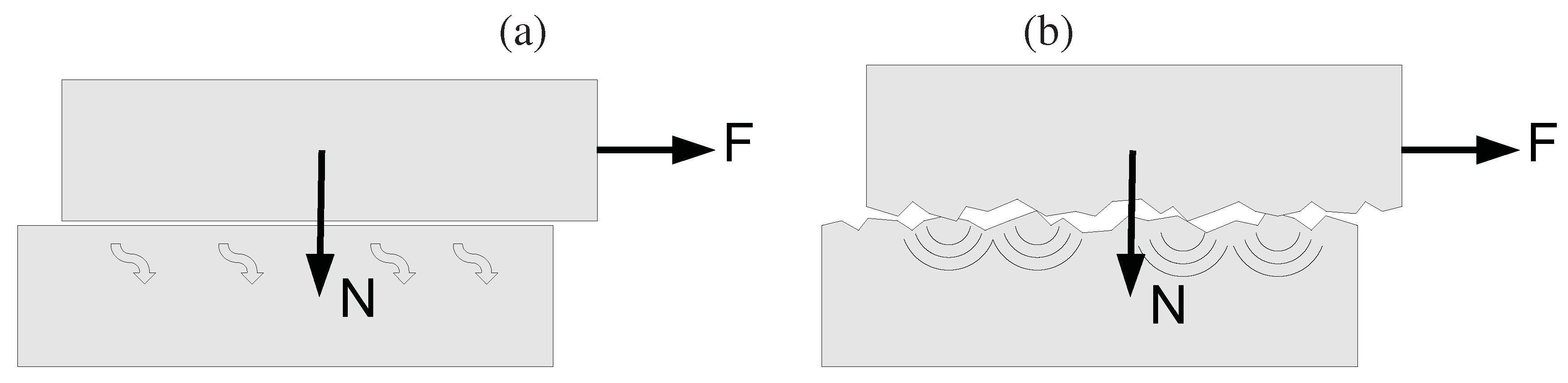
Finally, the transformation of mechanical work in audio vibration is realized by the friction noise phenomenon. For instance, when rubbing two metallic samples with rough surfaces [42,43] a noise is generated at the interface of samples. The basic phenomenon is that many light impacts occur between antagonist asperities and these impacts are responsible of the vibration in the samples which, in turn, radiate the sound. Since vibration is generated by light impacts which occur at any time and any location on the surface in a random manner, the source of sound can be considered as random and the resulting vibration as vibrational heat δQ > 0. The gain of vibrational entropy is therefore dS = δQ/T > 0 where T = E/kN. This is an irreversible process from the point of view of statistical vibroacoustics since work is transformed in vibrational heat. This is why it leads to an increase of vibrational entropy. A similar observation can be done for other types of contact noise such as instabilities in rubber/glass contact [44] or impact noise in gears [45].

Figure 7. (a) Friction is a conversion of mechanical energy into heat while (b) friction noise of rough surfaces is a conversion of a part of this mechanical energy into vibration.

Figure 7. (a) Friction is a conversion of mechanical energy into heat while (b) friction noise of rough surfaces is a conversion of a part of this mechanical energy into vibration.

These examples show that the difference between vibrational temperature and thermal temperature is not fundamental. In equilibrium situation when the mechanical system is at rest, both thermodynamical temperature and vibrational temperature are equal. But, in any situation where the mechanical structure is excited by external forces or sound, this equilibrium is broken and a large difference of temperatures can be observed. From this point of view, statistical vibroacoustics is the study of incoherent vibration when there is no equilibrium with thermal vibration (the situation of equilibrium with thermal range being a limit case). So, statistical energy analysis is the study of incoherent audio frequency vibrational energy. The vibrational power is injected by external forces or sound. Sub-systems can exchange vibrational energy and vibrational energy is also dissipated (a transformation of vibrational energy into heat).

Figure 8. Thermodynamics studies the transformation of work ∼0 Hz in thermal energy ∼10¹⁵ Hz. Statistical vibroacoustics focuses on energy which passes in audio frequency range ∼1 kHz.

Figure 8. Thermodynamics studies the transformation of work ∼0 Hz in thermal energy ∼10¹⁵ Hz. Statistical vibroacoustics focuses on energy which passes in audio frequency range ∼1 kHz.

6. Conclusions

The statistical approach applied to vibroacoustics is not fundamentally different from non-equilibrium thermodynamics. The concepts of vibrational temperature, vibrational heat and vibrational entropy and their relationships exactly match with the classical definitions and relationships in thermodynamics. We could say roughly that statistical vibroacoustics is nothing else than the application of thermodynamics to the audio frequency range. However, the possibility to do it with a certain efficiency is not trivial. In that concern, everything is possible because of Equation (2) states that random vibrational energy naturally flows from hot sub-systems to cool sub-systems, or, in other words, Clausius’ principle also applies in audio frequency range. It is important to note that this relationship cannot be demonstrated within the framework of statistical vibroacoustics. All the proposed demonstrations are based on the application of probability theory to the equations of mechanical resonators that is based on considerations on exact equations of motion. Equation (2) must rather be considered as the starting point of the statistical method in vibroacoustics in the same manner that Clausius’ principle is a postulate of classical thermodynamics.

References

- Rayleigh, J.W.S. The Theory of Sound. Two Volumes; Dover Publications Inc.: Toronto, Canada, 1945. [Google Scholar]
- Crighton, D.G. Acoustic beaming and reflexion from wave-bearing surfaces. J. Fluid Mech. 1971, 47, 625–638. [Google Scholar] [CrossRef]
- Davies, H.G. Natural motion of a fluid-loaded semi-infinite membrane. J. Acoust. Soc. Am. 1974, 55, 213–219. [Google Scholar] [CrossRef]
- Kompella, M.S.; Bernhard, R.J. Measurement of the statistical variation of structural-acoustic characteristics of automotive vehicles. In Proceedings of the Society of Automotive Engineers Noise and Vibration Conference, Warrendale, PA, USA, May 1993.
- Ben-Haim, Y. Set-models of information-gap uncertainty: Axioms and an inference scheme. J. Franklin Inst. 1999, 336, 1093–1117. [Google Scholar] [CrossRef]
- Lyon, R.H. Fluctuation theory and (very) early statistical energy analysis (SEA). J. Acoust. Soc. Am. 2003, 113, 2401–2403. [Google Scholar] [CrossRef] [PubMed]
- Lyon, R.H.; Maidanik, G. Power flow between linearly coupled oscillators. J. Acoust. Soc. Am. 1962, 34, 623–639. [Google Scholar] [CrossRef]
- Newland, D.E. Calculation of power flow between coupled oscillators. J. Sound Vib. 1966, 3, 262–276. [Google Scholar] [CrossRef]
- Scharton, T.; Lyon, R.H. Power flow and energy sharing in random vibration. J. Acoust. Soc. Am. 1968, 43, 1332–1343. [Google Scholar] [CrossRef]
- Gersh, W. Average power and power exchange in oscillators. J. Acoust. Soc. Am. 1969, 46, 118–1186. [Google Scholar] [CrossRef]
- Smith, P.W. Statistical models of coupled dynamical systems and the transition from weak to strong coupling. J. Acoust. Soc. Am. 1979, 65, 695–698. [Google Scholar] [CrossRef]
- Fahy, F.J.; De-Yuan, Y. Power flow between non-conservatively coupled oscillators. J. Sound Vib. 1987, 114, 1–11. [Google Scholar] [CrossRef]
- Newland, D.E. Power flow between a class of coupled oscillators. J. Acoust. Soc. Am. 1968, 43, 553–559. [Google Scholar] [CrossRef]
- Weaver, R.L. Equipartition and mean-square responses in large undamped structures. J. Acoust. Soc. Am. 2001, 110, 894–903. [Google Scholar] [CrossRef]
- Le Bot, A. Derivation of Statistical Energy Analysis from radiative exchanges. J. Sound Vib. 2007, 300, 763–779. [Google Scholar] [CrossRef]
- Maxit, L.; Guyader, J.L. Extension of SEA model to subsystems with non-uniform modal energy distribution. J. Sound Vib. 2003, 265, 337–358. [Google Scholar] [CrossRef]
- Shorter, P. Modeling noise and vibration transmission in complex systems. In Proceedings of IUTAM Symposium on the Vibration Analysis of Structures with Uncertainties, St Petersbourg, Russia, July 2009.
- Hynna, P.; Klindge, P.; Vuoksinen, P. Prediction of structure-borne sound transmission in large welded ship structures using statistical energy analysis. J. Sound Vib. 1995, 180, 583–607. [Google Scholar] [CrossRef]
- Craik, R.J.M. The prediction of sound transmission through buildings using statistical energy analysis. J. Sound Vib. 1982, 82, 505–516. [Google Scholar] [CrossRef]
- Sgard, F.; Nélisse, H.; Atalla, N.; Amedin, C.K.; Oddo, R. Prediction of the acoustical performance of enclosures using a hybrid statistical energy analysis: Image source model. J. Acoust. Soc. Am. 2010, 127, 784–795. [Google Scholar] [CrossRef] [PubMed]
- Langley, R.S. A derivation of the coupling loss factors used in statistical energy analysis. J. Sound Vib. 1990, 141, 207–219. [Google Scholar] [CrossRef]
- Totaro, N.; Dodard, C.; Guyader, J.L. SEA coupling loss factors of complex vibro-acoustics systems. J. Vib. Acoust. Trans. ASME 2009, 131, 041009-1. [Google Scholar] [CrossRef]
- Luzzato, E.; Ortola, E. The characterization of energy flow path in the study of dynamic systems in SEA theory. J. Sound Vib. 1988, 123, 189–197. [Google Scholar] [CrossRef]
- Tanner, G. Dynamical energy analysis—Determining wave energy distribution in vibro-acoustical structures in the high frequency regime. J. Sound Vib. 2009, 320, 1023–1038. [Google Scholar] [CrossRef]
- Fahy, F.J. Statistical energy analysis: A critical overview. In Statistical Energy Analysis: An Overview, with Applications in Structural Dynamics; Keane, A.J., Price, W.G., Eds.; Cambridge University Press: Cambridge, UK, 1997; pp. 1–17. [Google Scholar]
- Carcaterra, A. An entropy formulation for the analysis of energy flow between mechanical resonators. Mech. Syst. Sign. Process. 2002, 16, 905–920. [Google Scholar] [CrossRef]
- Le Bot, A. Entropy in Statistical Energy Analysis. J. Acoust. Soc. Am. 2009, 125, 1473–1478. [Google Scholar] [CrossRef] [PubMed]
- Jaynes, E.T. Information theory and statistical mechanics. Phys. Rev. 1957, 106, 620–630. [Google Scholar] [CrossRef]
- Uffink, J. Can the maximum entropy principle be explained as a consistency requirement? Stud. Hist. Phil. Modern Phys. 1997, 26B, 223–261. [Google Scholar] [CrossRef]
- Magionesi, F.; Carcaterra, A. Insights into the energy equipartition principle in undamped engineering structures. J. Sound Vib. 2008, 322, 851–869. [Google Scholar] [CrossRef]
- Carcaterra, A. Ensemble energy average and energy flow relationships for nonstationary vibrating systems. Special Issue Uncertainty in Structural Dynamics? J. Sound Vib. 2005, 288, 751–790. [Google Scholar] [CrossRef]
- Ferrari, C.; Guber, C. Friction force: From mechanics to thermodynamics. Euro. J. Phys. 2010, 31, 1159–1175. [Google Scholar] [CrossRef]
- Amiri, M.; Khonsari, M.M. On the thermodynamics of friction and wear—A review. Entropy 2010, 12, 1021–1049. [Google Scholar] [CrossRef]
- Rezek, Y. Reflections on friction in quantum mechanics. Entropy 2010, 12, 1885–1901. [Google Scholar] [CrossRef]
- Stolz, C. Thermodynamical description of running discontinuities: Application to friction and wear. Entropy 2010, 12, 1418–1439. [Google Scholar] [CrossRef]
- Nosonovsky, M. Entropy in Tribology: In the search for applications. Entropy 2010, 12, 1345–1390. [Google Scholar] [CrossRef]
- Kagan, E. Turing systems, entropy, and kinetic models for self-healing surfaces. Entropy 2010, 12, 554–569. [Google Scholar] [CrossRef]
- Fleurquin, P.; Fort, H.; Kornbluth, M.; Sandler, R.; Segall, M.; Zypman, F. Negentropy generation and fractality in the dry friction of polished surfaces. Entropy 2010, 12, 480–489. [Google Scholar] [CrossRef]
- Fox-Rabinovich, G.S.; Gershman, I.S.; Yamamoto, K.; Biksa, A.; Veldhuis, S.C.; Beake, B.D.; Kovalev, A.I. Self-Organization during Friction in Complex Surface Engineered Tribosystems. Entropy 2010, 12, 275–288. [Google Scholar] [CrossRef]
- Saulson, P.R. Thermal noise in mechanical experiments. Phys. Rev. D 1990, 42, 2437–2445. [Google Scholar] [CrossRef]
- Paolino, P.; Tiribilli, B.; Bellon, L. Direct measurement of spatial modes of a microcantilever from thermal noise. J. Appl. Phys. 2009, 106, 094313. [Google Scholar] [CrossRef] [Green Version]
- Le Bot, A.; Bou Chakra, E. Measurement of friction noise versus contact area of rough surfaces weakly loaded. Tribol. Lett. 2010, 37, 273–281. [Google Scholar] [CrossRef]
- Le Bot, A.; Bou Chakra, E.; Michon, G. Dissipation of vibration in rough contact. Tribol. Lett. 2010. [Google Scholar] [CrossRef] [Green Version]
- Deleau, F.; Mazuyer, D.; Koenen, A. Sliding friction at elastomer/glass contact: Inuence of the wetting conditions and instability analysis. Tribol. Int. 2009, 42, 149–159. [Google Scholar] [CrossRef]
- Perret-Liaudet, J.; Rigaud, E. Response of an impacting Hertzian contact to an order-2 subharmonic excitation: Theory and experiments. J. Sound Vib. 2006, 296, 319–333. [Google Scholar] [CrossRef] [Green Version]
© 2010 by the authors; licensee MDPI, Basel, Switzerland. This article is an open access article distributed under the terms and conditions of the Creative Commons Attribution license (http://creativecommons.org/licenses/by/3.0/).
Share and Cite
MDPI and ACS Style
Le Bot, A.; Carcaterra, A.; Mazuyer, D. Statistical Vibroacoustics and Entropy Concept. Entropy 2010, 12, 2418-2435. https://doi.org/10.3390/e12122418
AMA Style
Le Bot A, Carcaterra A, Mazuyer D. Statistical Vibroacoustics and Entropy Concept. Entropy. 2010; 12(12):2418-2435. https://doi.org/10.3390/e12122418
Chicago/Turabian StyleLe Bot, Alain, Antonio Carcaterra, and Denis Mazuyer. 2010. "Statistical Vibroacoustics and Entropy Concept" Entropy 12, no. 12: 2418-2435. https://doi.org/10.3390/e12122418